
PHY11006 Magnetism Notes#
Lecture 1:#
Key concepts: Magnetic fields are vector fields; magnetic charges (monopoles) do not exist; magnetic field lines are closed; the field is defined by the Lorentz force on a moving charge.
Magnetic fields, just like electric fields, are vector fields: they have both magnitude and direction at any point in space. As with electric fields, the direction of the magnetic field at a given point is shown by field lines, and the density of the field lines gives its strength. The field lines for the well-known case of a bar magnet are shown in Fig. 1(a). The field lines point away from N poles and towards S poles. A compass needle is a small, freely suspended bar magnet, which has a tendency to align with the field. (See Lecture 4). Hence the direction of a compass needle shows the direction of the field at any point in space. Magnetic field lines have tension, just like electric field lines, and from this you can explain the attraction and repulsion of magnetic poles.
The symbol for magnetic field is \(\mathbf{B}\). Note that this is a vector: the field strength is given by \(|\mathbf{B}|\), often just written \(B\), and the direction of \(\mathbf{B}\) gives the direction of the magnetic field. If the field has components \(B_x\), \(B_y\) and \(B_z\) along the \(x\), \(y\) and \(z\) axes, respectively, such that:
then
The SI unit of the \(\mathbf{B}\)-field is the Tesla, which is equivalent to N A-1 m-1. There is an older, non-SI unit of magnetic field that is still in widespread use called the Gauss, where 1 Gauss = T. For this reason, instruments to measure magnetic fields are often called “Gaussmeters” rather than “Teslameters”.
There are important differences between electric and magnetic fields. Both satisfy the same laws of electromagnetism, but the fields look and behave rather differently when they are static (i.e. constant in time.) This can be seen by comparing the magnetic field of a bar magnet shown in Fig. 1(a) with the electric field from a positive electric charge shown in Fig. 1(b). Here are two key differences:
Electric field lines start on positive changes and end on negative charges. Magnetic field lines, by contrast, always form closed loops.
A stationary positive test charge experience a force in the direction of the electric field. A stationary test charge experiences no force in a magnetic field.
Difference #1 is the consequence of the fact that, as far as we know, there are no “magnetic charges” that are equivalent to electric charges. It is not possible to find isolated N or S magnetic poles: they always come in pairs. If we chop a bar magnet in two, we end up with two smaller bar magnets, as shown in Fig. 2(a). In general, a single charge is called a monopole. Two separated equal and opposite charges \(+q\) and \(-q\) form an electric dipole, as, for example, in the Na+Cl- molecule. There are no magnetic monopoles: magnets always come as magnetic dipoles.
If you recall that electric field lines start and stop on electric monopoles, it becomes clear that the absence of magnetic monopoles means that magnetic field lines do not start or stop: they must always form closed loops. You might ask how this applies to Fig. 1(a), where the lines appear to start on the N pole and end on the S pole. The answer is that the field lines continue inside the magnet. The ones entering the S pole continue inside the magnet and emerge at the N pole.
Difference #2 follows from the fact that static electric charges do not experience a magnetic force in a magnetic field. The charge must be moving to experience a force. Experiments show that the force is perpendicular both to the velocity, \(\mathbf{v}\), of the charge and to \(\mathbf{B}\), as shown in Fig. 2(c). In S.I. units, the force on a moving charge \(q\) is defined as:
This force is called the Lorentz force. The direction of the force is worked out from the right-hand rule shown in Fig. 2(d). If there is also an electric field \(\mathbf{E}\) acting on the charge, then the total force will be given by:
The definition of \(\mathbf{B}\) given in eqn (1) is not all that convenient for measuring \(\mathbf{B}\). In practice, it is much simpler to make use of the fact that current-carrying wires contain moving charges, and to work out the force on the wire. We shall see how to do this is Lecture 3. The magnitude of \(\mathbf{B}\) can then be deduced from the force on the wire.
As a final difference between electric and magnetic fields, we note that:
Static charges do not generate a magnetic field. Magnetic fields are generated by moving charges.
The generation of electric fields by static electric charges is illustrated in Fig. 1(b). This static charge generates no magnetic field: the charge must be moving (e.g. in a current-carrying wire) to generate a magnetic field. We shall see how to calculate the fields generated by current-carrying wires in Lectures 5–7. One might naturally ask: where are the moving charges in the bar magnet shown in Fig. 1(a)? The simple answer is to say that the moving charges are the electrons circulating around the nuclei of the atoms, but the full answer is much more complicated, and involves the concept of electron spin. We shall leave that to a later Lecture.
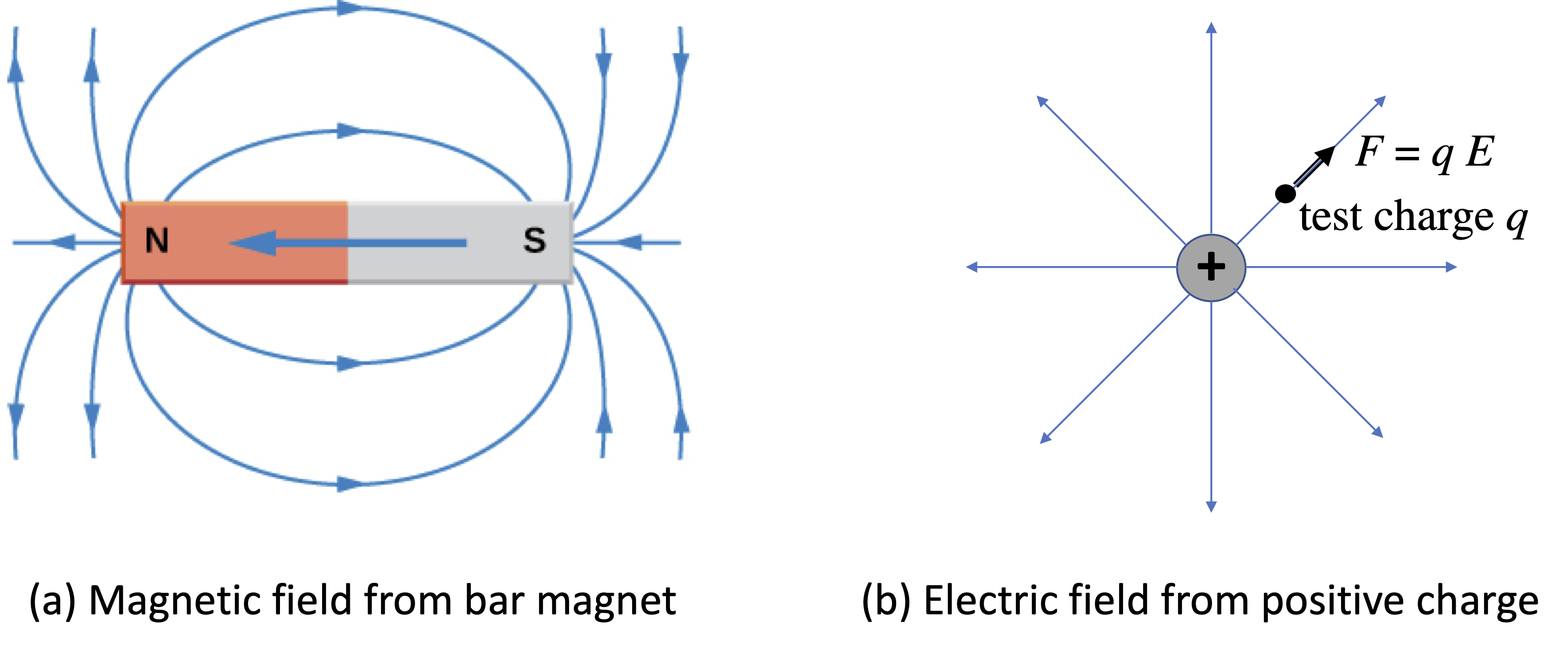
Fig. 1 (a) Magnetic field lines from a bar magnet. (b) Electric field lines from a positive charge. A test charge \(q\) in an electric field \(\mathbf{E}\) experiences a force given by \(\mathbf{F} = q \mathbf{E}\).#
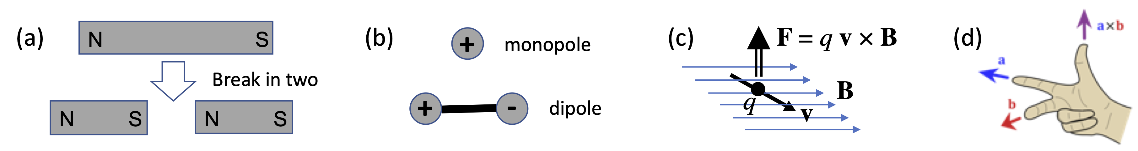
Fig. 2 (a) Magnets always come as pairs of N and S poles. (b) Two electric monopoles (i.e. charges) combine to form a dipole. (c) Lorentz force on a moving charge. (n.b. The force is downwards if \(q\) is negative.) (d) Right-hand rule for vector products.#
Lecture 2:#
Key concepts: Magnetic flux. Magnetic fields caused charged particles to undergo cyclotron motion.
Magnetic Flux#
Magnetic flux is defined in a very similar way to electric flux: it is the number of magnetic field lines piercing an area, or
If the field is normal to the surface, this definition simplifies to \(\Phi_B = BA\). The unit of magnetic flux is the (Wb), which is equivalent to T m2 or N m A-1. Since the magnetic field gives the flux per unit area, the magnetic field is sometimes called the magnetic flux density. Some older books also call the \(B\)-field the “magnetic induction”.
For an infinitesimal area d\(\mathbf{A}\), the flux is given by \(\rm{d} \Phi_B = \mathbf{B} \cdot \rm{d} \mathbf{A}\). Hence the magnetic flux over an arbitrary curved surface \(S\) becomes:
Note that this is not a closed surface, as in eqn (5) below. Since any field line that goes into a volume must also come out of that volume (i.e., all magnetic field lines are closed loops), only open surfaces can have non-zero magnetic flux.
In electrostatics, Gauss’s law states that the integral of the electric field over a closed surface is equal to \(Q_{\rm total}/ \epsilon_0\). Since there are no magnetic monopoles, the equivalent of Gauss’ law for magnetic fields is
This is again a universally valid law of nature, but it does not really help us calculating the magnetic field like Gauss’ law did for the electric field.
Cyclotron motion#
In the previous lecture we saw that the magnetic force on a charge with velocity \(\mathbf{v}\) is given by:
Due to the cross product, the Lorentz force always points perpendicular to both the particle’s velocity direction and the magnetic field. This means that along the trajectory of the particle the Lorentz force does not do any work \(W\):
since \(\mathbf{v}\) and \(\rm{d}\mathbf{l}\) point in the same direction. This means that the kinetic energy of the particle is unchanged, and so its speed is constant.
However, the velocity is changing all the time as the particle is deflected by the magnetic force.
Consider a positively charged particle moving with velocity \(\mathbf{v}\) perpendicular to \(\mathbf{B}\), as shown in Fig. 3(a). The × symbols represent a \(\mathbf{B}\)-field pointing in to the page. (A field pointing out of the page is shown by a \(\bullet\) symbol. Think of an arrow: a point means that the arrow is coming towards you, while tail feathers imply motion away from you.) The force is perpendicular to both \(\mathbf{v}\) and \(\mathbf{B}\) and has magnitude \(F=qvB\). This produces circular motion, with radius \(R\) given by:
The circular path of a charged particle in a perpendicular magnetic field is called cyclotron motion. The cyclotron radius \(R\) is equal to \(m v / q B\), and the period \(T\) is \(2\pi R /v = 2 \pi m / qB\). Hence the cyclotron frequency is \(q B / 2 \pi m\), and the cyclotron angular frequency \(\omega_{\rm c}\) is \(q B / m\). Note that these do not depend on \(v\). In the case of a negatively charged particle, we replace \(q\) by \(|q|\) in all these formul, and note that the sense of the rotation is reversed. Thus positive particles rotate in an anticlockwise sense in Fig. 3(a), while negative particles would rotate in a clockwise sense.
When the field and velocity are not perpendicular to each other, charged particles follow a helical path as shown in Fig. 3(b). We resolve the velocity \(\mathbf{v}\) into components \(v_\perp\) and \(v_\parallel\), which are perpendicular and parallel to \(\mathbf{B}\), respectively. The radius of the helix is determined by the perpendicular component, with \(R= m v_\perp / |q| B\), and the particle moves along the axis of the helix with the speed of the parallel component, \(v_\parallel\). Hence the pitch of the helix is \(v_\parallel T\).
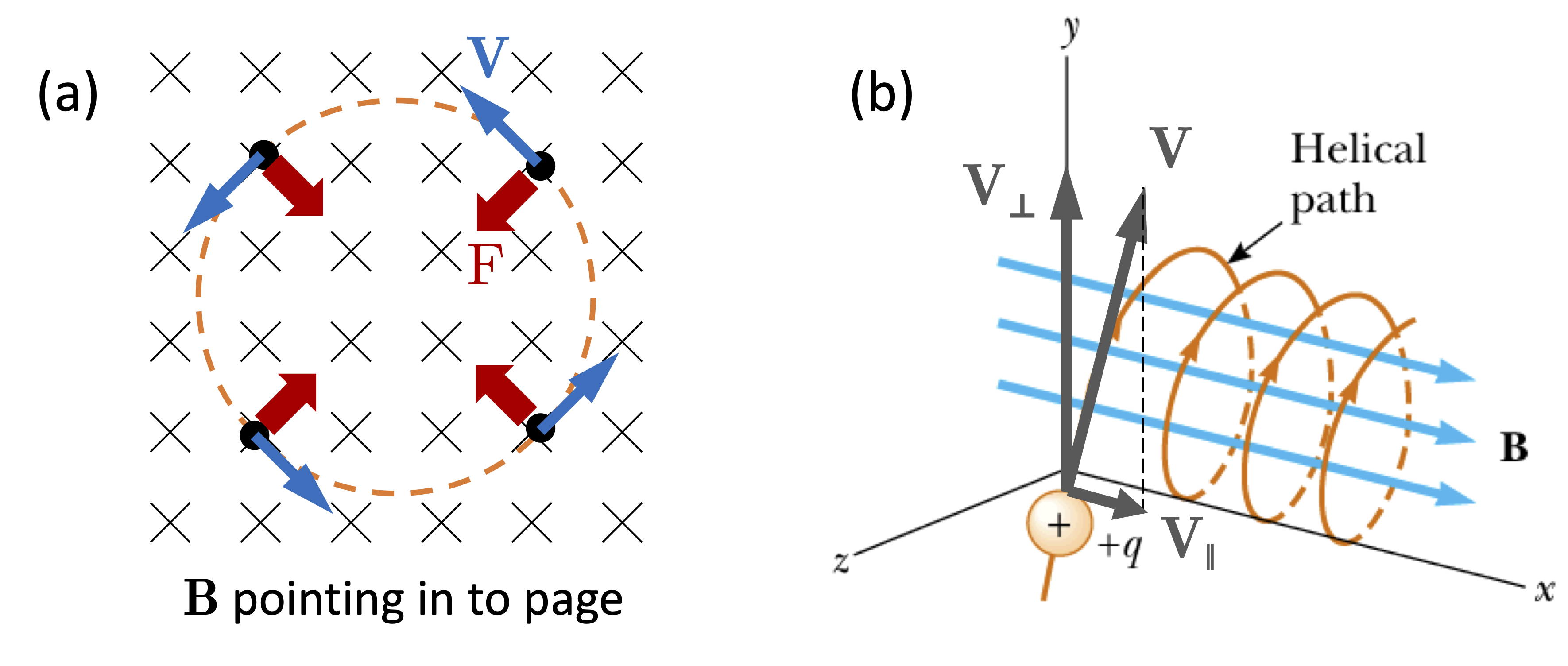
Fig. 3 (a) Cyclotron motion of a positively charged particle moving in a perpendicular field. The × symbols signify the field pointing in to the page. Negatively charged particles follow a circular path with the opposite sense. (b) Helical motion for a particle with a velocity component along the field direction.#
Lecture 3:#
Key concepts: The Lorentz force on a current-carrying wire is independent of the sign of the charges. The Hall effect provides a convenient basis for measuring magnetic fields. Magnetic dipoles are defined in terms of current loops. In a uniform magnetic field, the Lorentz force on a magnetic dipole creates a torque, but no net force.
Let us consider the magnetic force on a current-carrying wire in a perpendicular \(\mathbf{B}\)-field as shown in Fig. 4(a). For the sake of simplicity at this stage, we assume that the particles that carry the current are positively charged. Consider a small, straight section of wire with area \(A\) and length \(L\) carrying a current \(I\). The total number of charges is equal to \(n A L\), where \(n\) is the number of charges per unit volume. The charge per unit time (i.e. the current \(I\)) is thus:
where \(v\) is the drift velocity of the charges. For future reference, we note that the current per unit area (usually called the current density or current flux with symbol \(J\)) is given by:
Each charge experiences a Lorentz force of \(q v B\) which is perpendicular to \(\mathbf{v}\) and \(\mathbf{B}\), and hence the total force on the wire is \(n A L qvB\). On inserting from eqn (7), we see that \(F=ILB\). If the field is not perpendicular to the wire, we need to take its perpendicular component, namely \(B \sin \theta\), where θ is the angle between the wire and the field. We thus see that we can write the Lorentz force on a small line segment \(\rm{d}\mathbf{l}\) of current-carrying wire as
For a line segment of length \(L\) in the direction \(\hat{\mathbf{l}}\), this becomes \(\mathbf{F} = IL\,\hat{\mathbf{l}}\times \mathbf{B}\). Note that, although we assumed that \(q\) was positive for simplicity, the direction of the force does not depend on the sign of the charge; if \(q\) is negative, then \(\mathbf{v}\) has to be in the opposite direction for a given current direction, and hence the direction of \(\mathbf{F}\) remains unaltered. Note also that eqn (9) provides a more convenient way to measure \(B\) than the more basic form of the Lorentz force in eqn (6).
The Hall effect considers a current passing through a slab rather than a thin wire. In the wire, the charges are constrained to move in the direction of the wire, but this is not the case for a slab, where the charges can be deflected. We consider the geometry where the current flows in the \(x\) direction and the \(\mathbf{B}\)-field is applied in the \(y\) direction, as shown in Fig. 4(b). In this situation, the current-carrying charges experience a force in the \(z\) direction. The deflected charges accumulate on one side of the slab, which generates an electric field \(E_z\) in the \(-z\) direction. This opposes the magnetic force, and equilibrium is reached (see eqn (2)) when \(E_z = -v_x B_y\). This can be re-written in terms of the current density \(J_x\), the charge carrier density \(n\) and the charge \(q\) as:
\(E_z\) is determined by measuring the Hall voltage (see \(V_0\) in Fig. 4(b)) that develops along the \(z\) direction in a sample of known dimensions. Measurements of the Hall effect enable the charge carrier density \(n\) to be determined.
A measurement of the Hall voltage in a material of known carrier density carrying a calibrated current provides a sensitive probe of the magnetic field. This is the basis of Hall probes used for field measurements.
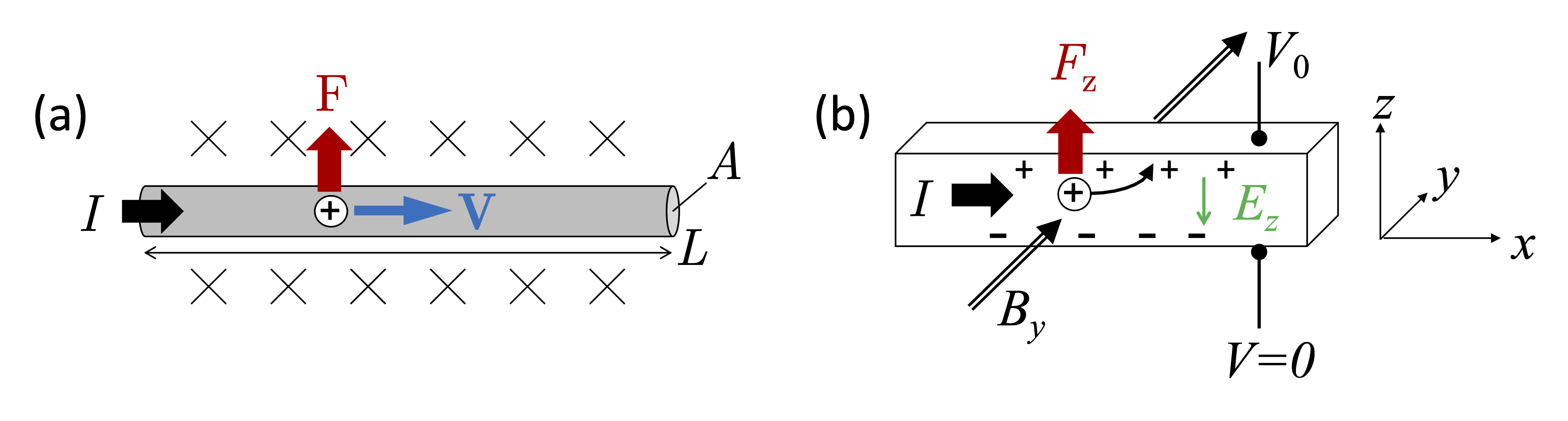
Fig. 4 (a) Force on the current-carrying charges (assumed positive) in a wire. The magnetic field \(B\) points in to the page. (b) The Hall effect.#
We have seen above that the Lorentz force on a small line segment \(\rm{d}\mathbf{l}\) of current-carrying wire is given by eqn (9). We now consider the forces on current-carrying loops. We shall see that this naturally leads us to the key concept of the magnetic dipole moment. Since there are no magnetic monopoles, the magnetic dipole is the principal building block for magnetic materials. Hence the definition of the magnetic dipole moment is central to the theory of magnetism.
Consider a rigid rectangular closed loop with sides of length \(a\) and \(b\) carrying a current \(I\). The loop is placed in a uniform magnetic field \(\mathbf{B}\), as shown in Fig. 5(a). Each side \(j\) of the loop experiences a Lorentz force given by eqn (9).
where \(\mathbf{l}_j\) is the vector that encodes the direction and length of side \(j\). We define θ as the angle between the normal vector \(\hat{\mathbf{n}}\) of the loop and \(\mathbf{B}\), such that the forces on the four sides of the loop are given by: The total force is thus:
which show that there is no net force on the loop.
Now consider the torque about the axis O parallel to the \(x\) axis as shown in Fig. 5(b). The end wires 1 and 3 produce no torque as the force is parallel to the axis. Wires 2 and 4, by contrast, do produce a torque, as they both tend to turn the loop in the clockwise direction. The torque produced by \(\mathbf{F}_2\) and \(\mathbf{F}_4\) is calculated as:
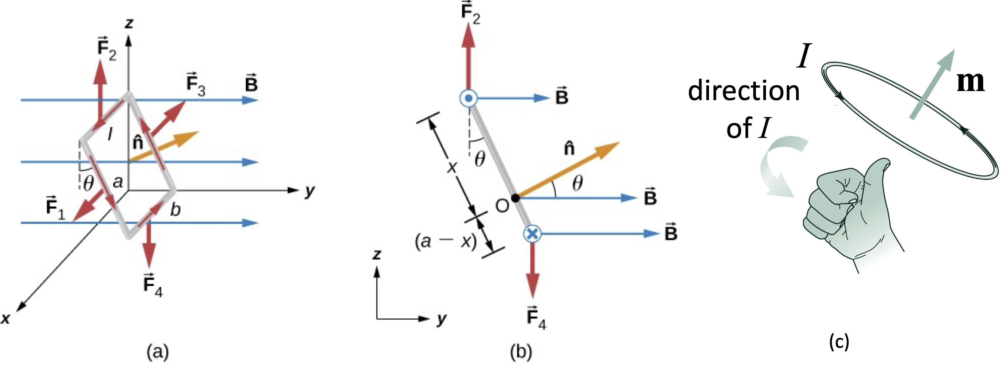
Fig. 5 (a) A current carrying loop in a magnetic field. (b) Side view showing the turning forces about the axis O. (a) Right-hand rule for magnetic dipoles.#
We now introduce the magnetic dipole moment \(\mathbf{m}\) defined by:
where \(\mathbf{A}\) is a vector in the direction of \(\hat{\mathbf{n}}\) with magnitude equal to the area of the surface enclosed by the loop. It is most conveniently represented by a thumbtack vector, and it is not restricted to regularly-shaped loops. The direction of \(\mathbf{m}\) is determined by the right-hand rule on the current loop, as shown in Fig. 5(c).
On noting that \(A=ab\) so that \(|\mathbf{m}|=Iab\), we see that the torque is \(|\mathbf{m}| B \sin \theta \, \hat{\mathbf{i}}\), which implies that:
This is analogous to the torque on an electric dipole in an electric field: \(\mathbf{\tau} = \mathbf{p}\times\mathbf{E}\).
Lecture 4:#
Key concepts: Electric motors. Magnetic dipoles tend to align with the field. Energy of magnetic dipoles in magnetic fields. Force on a magnetic dipole in a non-uniform field.
In the last lecture we introduced the key concept of the magnetic dipole moment \(\mathbf{m}\) and showed that the torque in a uniform field is equal to \(\mathbf{m}\times \mathbf{B}\). (see eqn (11).) In this lecture we derive more important results for magnetic dipoles.
The torque on the dipole is maximized when \(\mathbf{m}\) and \(\mathbf{B}\) are orthogonal (i.e. \(\theta = 90^\circ\)), where we have \(|\mathbf{\tau}| = |\mathbf{m}| B\). The torque is zero for \(\theta = 0\) and \(\theta = 180^\circ\), and switches sign for \(180^\circ < \theta < 360^\circ\). The means that the loop will always tend to align with \(\mathbf{m}\) parallel to \(\mathbf{B}\) (i.e. \(\theta = 0\)), where the torque is zero. Magnetic dipoles therefore have the tendency to line up in a magnetic field. If we start in this equilibrium position with \(\theta = 0\), and rotate the dipole either way, the torque will tend to turn the loop back to its equilibrium position, performing damped oscillations as indicated in Fig. 6(a).
To prevent these oscillations and get continuous torque that can be used in a DC electric motor, the direction of the current (and hence \(\mathbf{m}\)) has to be switched every \(180^\circ\) in order to maintain the direction of the torque. This is done by using a commutator, as shown in Fig. 6(b). Since the torque is proportional to \(|\mathbf{m}|\), practical motors usually use a coil instead of a single loop. A coil with \(N\) turns is equivalent to \(N\) loops, and hence has a magnetic dipole moment of \(NIA\).
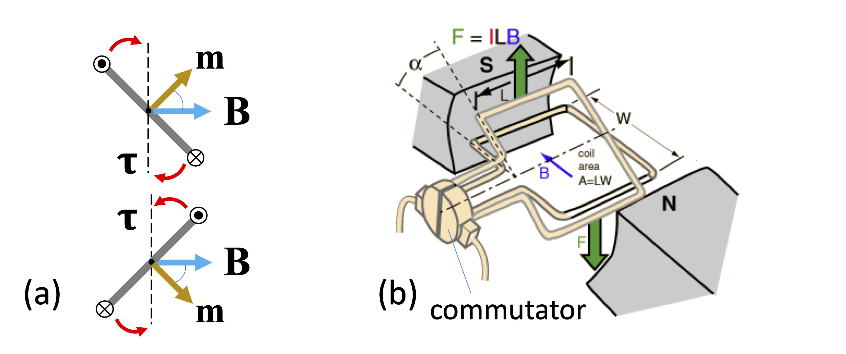
Fig. 6 (a) Oscillations of a magnetic dipole about the equilibrium position with \(m\) parallel to \(\mathbf{B}\). (b) DC electric motor incorporating a commutator.#
Let us now work out the energy of a magnetic dipole in a magnetic field. We have seen in Lecture 2 that the Lorentz force \(\mathbf{F}\) on a charged particle moving with velocity \(\mathbf{v}\) in a magnetic field \(\mathbf{B}\) is perpendicular to the direction of \(\mathbf{v}\) on account of the cross product \(\mathbf{F} = q\mathbf{v}\times\mathbf{B}\), and hence that the work \(\mathbf{F}\cdot\mathbf{d}\) done on a particle as it moves through the field is zero. However, there is work being done on a magnetic dipole as we rotate it in an external field:
Now \(\tau = \mathbf{m}\times \mathbf{B} = m B \sin\theta\), and so we have:
This means that the magnetic energy \(U_{\mathbf{m}}\) stored in the dipole is equal to \(- \mathbf{m}\cdot \mathbf{B} + C\). In analogy with electric dipoles, we define the zero of energy when \(\theta = \pi/2\) (i.e. when the dipole and the field are perpendicular), which implies that \(C=0\). The magnetic energy of a magnetic dipole in a uniform magnetic field is thus given by:
Note that \(U_{\mathbf{m}}\) has a minimum value of \(-mB\) when \(\mathbf{m}\) is parallel to \(\mathbf{B}\) and a maximum value of \(+mB\) when it is anti-parallel. Note also that this is of the same form as the energy of an electric dipole in an electric field which is given by \(U = - \mathbf{p} \cdot \mathbf{E}\).
We have seen in Lecture 3 that the force on a magnetic dipole in a uniform field is zero. However, this is not the case if the field is non-uniform. In this case we can work out the force from the negative gradient of the potential energy:
If the field is just in one direction (say the \(z\)-direction), the force is along the direction of the field gradient and is given by:
This is an important result for understanding the Stern–Gerlach experiment in quantum mechanics.
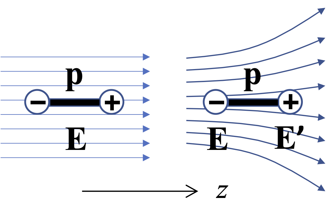
Fig. 7 Comparison of an electric dipole in uniform and non-uniform fields. The dipole is taken to be oriented along the \(z\) direction.#
The results for the force in the non-uniform field can be understood by analogy with an electric dipole. In Fig. 7 we have a dipole \(\mathbf{p}\) in a uniform electric field \(\mathbf{E}\) pointing in the \(z\) direction. The force on the positive and negative charges are \(+QE_z\) and \(-QE_z\) respectively, and so the total force on the dipole is zero. On the other hand, if the field is non-uniform, as shown on the right of Fig. 16(a), the forces are not the same. The force on the negative charge is \(-QE_z\), while that on the positive charge is \(+QE_z'\), giving a net force \(F_z\) of \(Q(E_z'-E_z)\). On writing \(E_z'\) as
where \(d\) is the separation of the charges, and noting that \(p_z= Qd\), we see that
This is of the same form as eqn (14). The close analogy between the results for electric and magnetic dipoles is summarized in Table 1.
Electric |
Magnetic |
|
Definition |
\(\mathbf{p} = q \mathbf{d}\) |
\(\mathbf{m}= I \mathbf{A}\) |
Units |
C m |
A m2 |
Energy |
\(U=-\mathbf{p} \cdot \mathbf{E}\) |
\(U=-\mathbf{m}\cdot \mathbf{B}\) |
Torque |
\(\mathbf{\tau}= \mathbf{p} \times \mathbf{E}\) |
\(\mathbf{\tau} = \mathbf{m}\times \mathbf{B}\) |
Force in uniform field |
0 |
0 |
Force in non-uniform field |
\(F_z=p_z \frac{{\rm d} E_z}{ {\rm d} z}\) |
\(F_z=m_z \frac{ {\rm d} B_z}{ {\rm d} z}\) |
Lecture 5:#
Key concepts: Generation of fields by moving charges. Calculation of the magnetic field due to a current element by Biot–Savart’s law. Magnetic field from a straight wire.
We noted in Lecture 1 that only moving charges generate a magnetic field. This was first discovered by Oersted in 1820, when he observed the deflection of compass needles near current-carrying wires. These experiments showed that the direction of the field is perpendicular to the velocity of the moving charges and falls off quadratically with distance. The field produced at position \(\mathbf{r}\) relative to a charge moving with velocity \(\mathbf{v}\) can therefore be written:
where \(\hat{\mathbf{r}}=\mathbf{r}/r\) is a unit vector in the direction of \(\mathbf{r}\). The proportionality constant \(\mu_0\) is the magnetic permeability of free space, and has a value that is very close to \(4 \pi \times 10^{-7}\) Wb A-1 m-1 in S.I. units. (Alternative units are T m A-1 or N A-2.)
Equation (15) is not very useful, as we rarely try to generate magnetic fields using free charged particles. Instead, we use current-carrying wires. There is no such thing as a ‘point’ current that is analogous to a ‘point’ charge in electrostatics, since a current must flow around a closed circuit. Nevertheless, we can express the infinitesimal contribution to the magnetic field \(\rm{d}\mathbf{B}\) at a position in space \(\mathbf{R}\) due to an infinitesimal line element \(\rm{d}\mathbf{l}\) at position \(\mathbf{R}'\) carrying a current \(I\) as
The arrangement of the various vectors is shown in figure 8(a). To find the total magnetic field, we add up all the infinitesimal parts:
where the path \(C\) is the line along which the current flows. These tend to be challenging integrals, and should include all the current-carrying wires to find the total magnetic field, but they do not rely on special symmetries like the method using Ampere’s law.
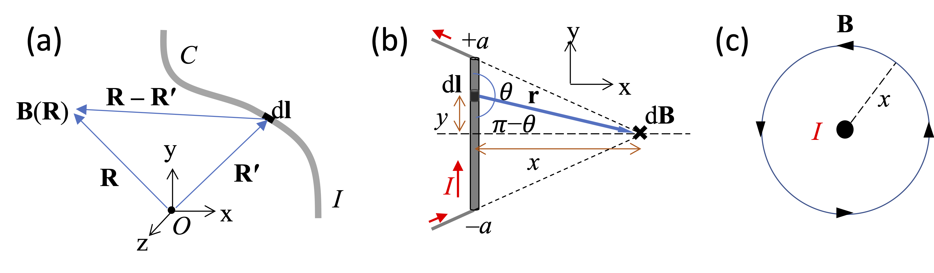
Fig. 8 (a)The definition of the vectors in the law of Biot and Savart for a wire following a path \(C\) carrying a current \(I\). The line element \(\rm{d}\mathbf{l}\) points in the direction of the current. Note that the origin \(O\) is necessary to make sense of \(\mathbf{R}\) and \(\mathbf{R}'\), but the relevant distance \(\mathbf{R}'-\mathbf{R}\) between the line segment and the point where we evaluate the magnetic field is independent of \(O\). (b) Calculation of the field produced by a straight wire of length \(2a\). (c) Magnetic field line looping around the wire, following the right-hand thumb rule.#
Often, the role of the origin is not mentioned explicitly, and the Biot–Savart law is expressed in terms of the vector from the current element to the position of interest, namely \(\mathbf{r} = \mathbf{R}-\mathbf{R}'\):
and
The integral is evaluated over the whole wire.
As an example, we consider the field produced by a straight current-carrying wire of length \(2a\), as shown in Fig. 8(b). The wire is orientated along the \(y\) axis, and runs from \(y=-a\) to \(y=+a\). Our goal is to calculate the field produced at position \((x,0,0)\), which lies a distance \(x\) from the centre of the wire, using eqn (17). The wire carries a current \(I\), which enters and leaves via wires that aim at \((x,0,0)\). Since \(\rm{d}\mathbf{l}\) is parallel to \(\mathbf{r}\) in these end wires, they produce no field, as \(\rm{d}\mathbf{l} \times \mathbf{r} = 0\). We therefore only have to consider the current elements running from \(y=-a\) to \(+a\).
Consider a current element \(\rm{d}\mathbf{l}\) at position \((0,y,0)\), as shown in Fig. 8(b), so that \(\rm{d} \mathbf{l} = \rm{d} y \hat{\mathbf{j}}\). The vector \(\mathbf{r}\) points from \(\rm{d}\mathbf{l}\) at \((0,y,0)\) to \((x,0,0)\). We therefore have \(\mathbf{r} = (x,-y,0)\), and hence \(r^2 = x^2+y^2\). The vector \(\rm{d}\mathbf{l} \times \hat{\mathbf{r}}\) points in the \(-z\) direction, as indicated by the × symbol at \((x,0,0)\) in Fig. 8(b). Now \(|\rm{d}\mathbf{l} \times \hat{\mathbf{r}}| = \rm{d} l \sin \theta\), where θ is the angle between \(\rm{d} \mathbf{l}\) and \(\mathbf{r}\), and \(\sin \theta = \sin (\pi-\theta) = x/r\). We thus get:
Hence, with \(r= (x^2+y^2)^{1/2}\), we get:
which implies that the field strength \(B \equiv | \mathbf{B}|\) is given by:
The field lines loop around the wire according to the right-hand thumb rule as shown in Fig. 8(c), and the field drops off as \(1/|x|^2\) at large \(x\), where \(|x| \gg a\).
We can find the field from a long straight wire by letting \(a \rightarrow \infty\) in eqn (18). The final result is:
Notice how the magnetic field drops off as \(1/x\), which is the same as for the electric field from a straight line charge.
Lecture 6:#
Key concept: Forces between current-carrying wires. Fields from loops and coils.
We have seen in the previous lecture that the field produced at a distance \(r\) by a long, straight wire carrying a current \(I\) is given by (see eqn (19) with \(x=r\)):
The field lines loop around the wire, following a right-hand rule, as shown in Fig. 9(a). We have also seen previously that the force on a current-carrying element \(\rm{d} \mathbf{l}\) is given by (see eqn (9)):
We can combine these two results to work out the force between two infinite, parallel, current-carrying wires. Consider two such wires, as shown in Fig. 9(b). We can find the force per unit length either by calculating the force \(F_{21}\) on wire 2 due to the field produced by wire 1, or by calculating the force \(F_{12}\) on wire 1 due to the field from wire 2. Let us work out \(F_{21}\) first. The Field \(B_1\) from wire 1 at wire 2 points into the page (the \(-z\) direction) and has magnitude \(B_1 = \mu_0 I_1 / 2 \pi r\). The current elements in wire 2 point along \(y\), and so \(\rm{d} \mathbf{l} \times \mathbf{B}\) is in the \(-x\) direction. Hence the force on a length \(L\) of wire 2 is given by
Similarly, \(F_{12} = I_1 L B_2 = (\mu_0I_1 I_2/2 \pi r)L\). We thus conclude that the force per unit length between two long, parallel wires carrying currents \(I_1\) and \(I_2\) and separated by a distance \(r\) is given by:
The force is attractive if the currents are in the same direction, and repulsive if they are in opposite directions. If we take \(\mu_0=4 \pi \times 10^{-7}\) Wb A-1 m-1, then we get a force of \(2 \times 10^{-7}\) N when a current of 1 Ampere flows through both wires and the separation is 1 m. This is the old definition of the Ampere, but the definition has now been changed,
and the force is now only approximately \(2 \times 10^{-7}\) N to within a fractional accuracy of about \(10^{-10}\).
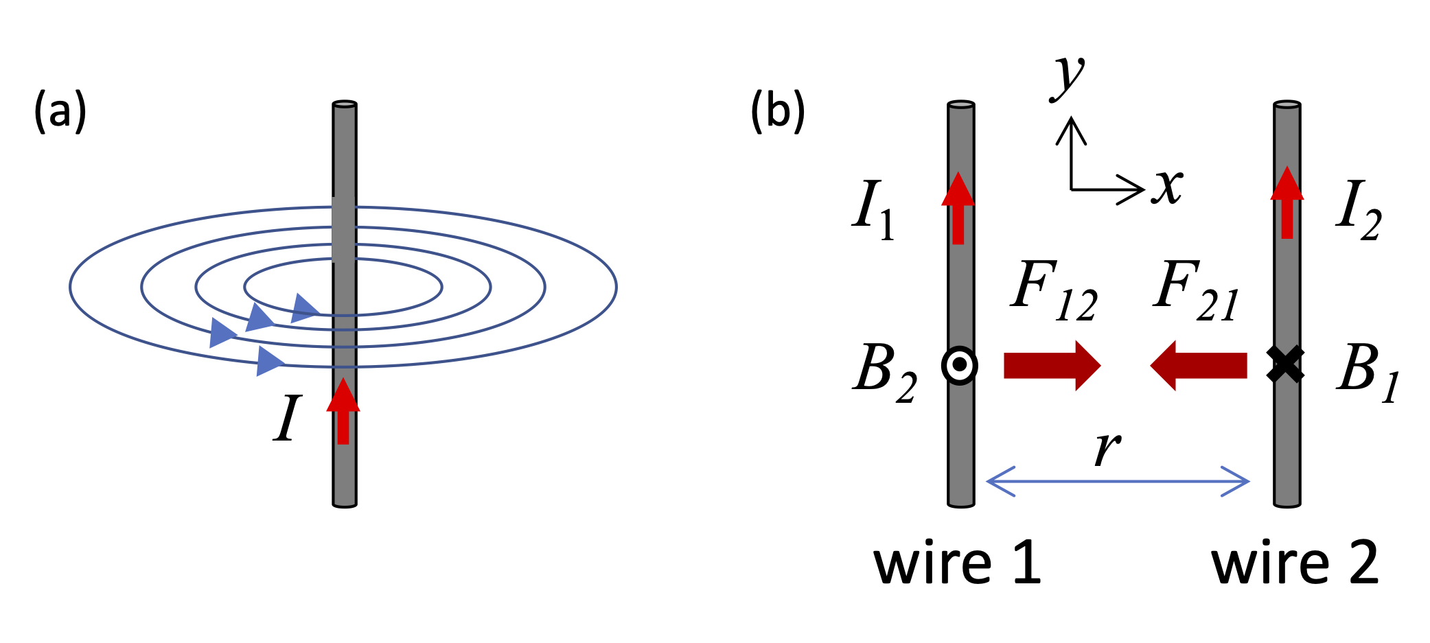
Fig. 9 (a) Field lines for a long current-carrying straight wire. (b) Two parallel current-carrying wires separated by a distance \(r\).#
As another example of Biot–Savart’s law, we can find the field produced by a current loop along its axis. Consider a loop of radius \(a\) carrying a current \(I\), as shown in Fig. 10(a). We start by finding the field produced by a current element \(\rm{d} \mathbf{l}\) at the top of the loop. In the co-ordinate frame of Fig. 10(a), which has its origin at the centre of the loop, \(\rm{d} \mathbf{l}\) points along the \(z\) axis, while \(\mathbf{r}\) points from \(\rm{d} \mathbf{l}\) to \((x,0,0)\), and is given by \(\mathbf{r} = (x,-a,0)\). The direction of \(\rm{d} \mathbf{l} \times \hat{\mathbf{r}}\) lies in the \(xy\) plane, making an angle \((\pi/2-\theta)\) with the \(x\) axis, where θ is defined in the figure. Note that \(\mathbf{r}\) is perpendicular to \(\rm{d} \mathbf{l}\), so that \(|\rm{d} \mathbf{l} \times \hat{\mathbf{r}}| = \rm{d} l\). From Biot–Savart’s law, we then get two components:
Let us consider the off-axis component \(\rm{d} B_y\) first. On rotating \(\rm{d} \mathbf{l}\) around the loop, the direction of \(\rm{d} \mathbf{l} \times \hat{\mathbf{r}}\) rotates around the axis with it, so that the off-axis components cancel out when added all together. We therefore only have a net contribution from \(\rm{d} B_x\), which is the same for all current elements around the loop. On recalling that \(\cos (\pi/2-\theta) = \sin \theta\) and integrating around the loop, we get:
On noting that \(r=\sqrt{a^2+x^2}\) and that \(\sin \theta = a/r\), we get the final result:
The field has a maximum value of \(\mu_0 I / 2 a\) at \(x=0\), and falls off symmetrically with increasing \(|x|\). For large \(|x|\), where \(|x| \gg a\), the field falls off as \(1/|x|^3\). The field pattern is shown in Fig. 10(b). The field from a single loop is fairly small, and so practical electromagnets use coils instead. In a coil we wrap the wire around the loop \(N\) times, effectively giving \(N\) loops. The fields from the loops add together, increasing the field strength by a factor of \(N\).
We noted in Lecture 3 that a current loop gives a magnetic dipole moment \(m\) equal to \(IA\). In the case of a circular loop, we have \(m=I \pi a^2\), and we can rewrite eqn (21) as:
This makes the \(1/|x|^3\) dependence at large \(x\) an expected result, as dipole fields fall off as \(1/r^3\) rather than \(1/r^2\).
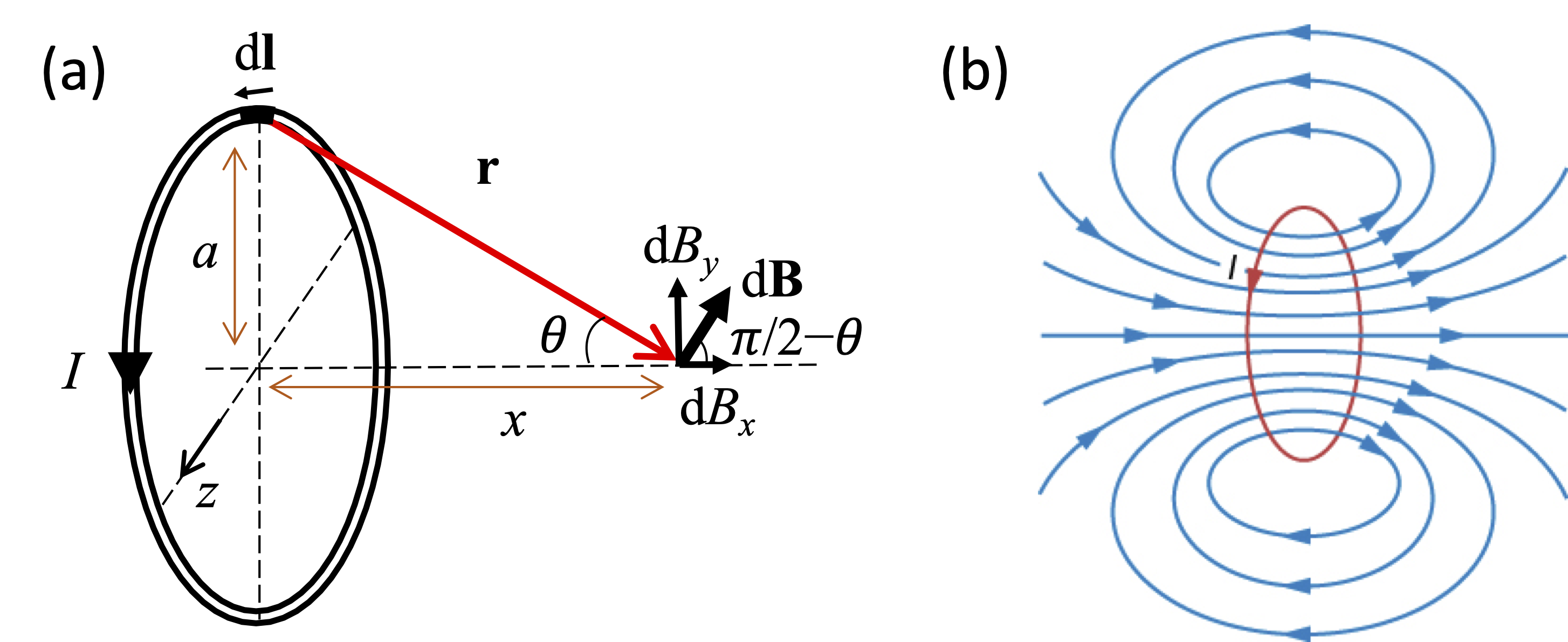
Fig. 10 (a) Field at distance \(x\) along the axis of a circular loop of radius \(a\) carrying a current \(I\). (b) Field lines from the current loop.#
Lecture 7:#
Key concept: Ampere’s law gives a method for calculating magnetic fields, analogous to Gauss’ law in electrostatics.
Ampere’s law states that the path integral of the field around a closed loop is equal to \(\mu_0\) times the total current enclosed by the loop:
We can write \(I_{\rm enclosed}\) as the integral of the current density over any surface \(S\) bounded by \(C\):
Ampere’s law is valid only when there are no time-varying electric fields around. It can be used to calculate the magnetic field due to a current in much the same way Gauss’ law helped us calculate the electric field. Since Ampere’s law is true for any surface \(S\) with boundary \(C\), you can choose \(S\) and \(C\) based on the symmetry of the problem. We consider three examples below.
Long straight wire#
Consider a straight wire carrying a current \(I\). By cylindrical symmetry, the magnetic field must have constant magnitude on the surface of any cylinder centred around the wire with radius \(r\). Since we also know that the magnetic field lines must be closed, they cannot originate on the wire, and more generally, they cannot be radially outward. The only other way that respects the cylindrical symmetry is when the field lines are circular loops around the wire, as shown in Fig. 11(a). In that case, the tangent line element \(\rm{d}\mathbf{l}\) lies in the same direction as (or opposite to) the magnetic field lines, and the dot product \(\mathbf{B}\cdot\rm{d}\mathbf{l}\) is just equal to \(B\, \rm{d} l\). With \(B\) constant around the loop \(C\), we find
where the line integral was evaluated over the circumference of a circle with radius \(r\). We then find that the magnitude of \(B\) is given by:
This is identical to the result derived by Biot–Savart’s law, as it must be, (see eqn (20)), but the derivation is much simpler.
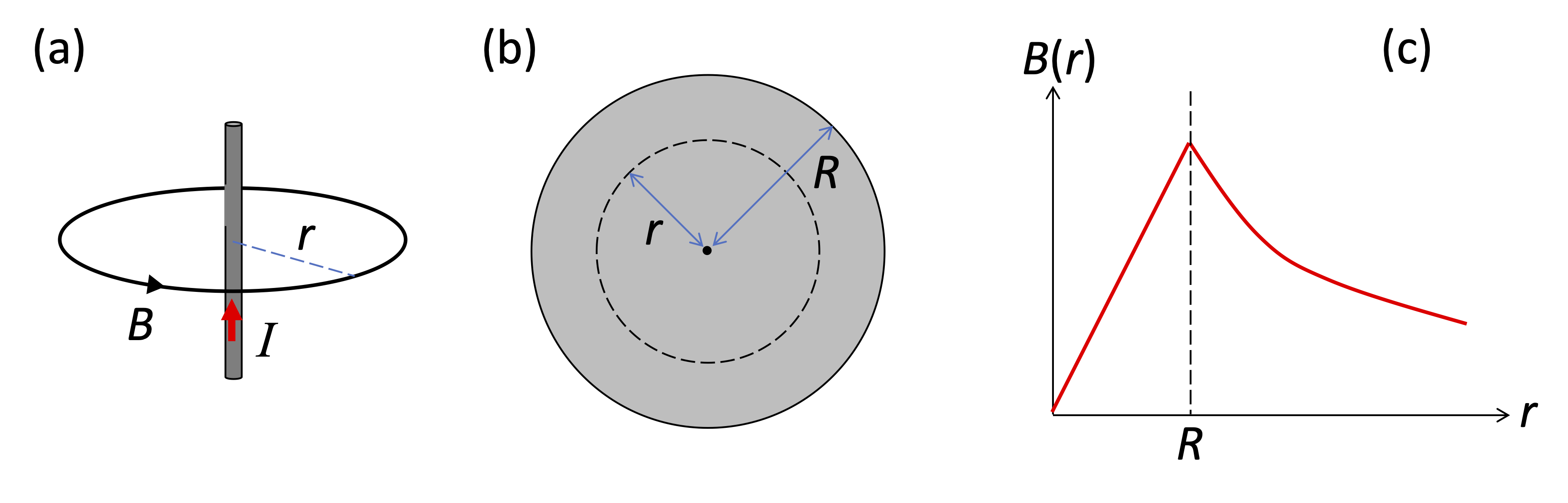
Fig. 11 (a) Magnetic field from a wire carrying a current \(I\). (b) Amprian loop within a wire of finite radius \(R\). (c) Variation of \(B\) with distance \(r\) from the centre of the wire.#
Field inside a wire#
We now consider the magnetic field inside a long straight wire of finite radius, \(R\). We assume that the current, \(I\), flows uniformly through the wire, so that the current density \(J\) (i.e. current per unit area, with units A m-2) is given by:
We choose an Amperian loop of radius \(r\) around the centre of the wire, as shown in Fig. 11(b). The current enclosed within the Amperian loop is equal to \(J * \pi r^2\), which implies \(I_{\rm enclosed}= Ir^2/R^2\). We thus have from Ampere’s law (eqn (22)):
We could also have obtained this from eqn (23). We conclude that the field is given by:
The field thus increases linearly with radius up to the edge of the wire, as shown in Fig. 11(c). When \(r=R\), the field has its maximum value of \(\mu_0 I/2 \pi R\), which is consistent with eqn (24). For \(r>R\), the field decays according to eqn (24), since we are now outside the wire.
Solenoids#
Our last example is a solenoid. This is a wire that wraps around itself as a helix, as shown in Fig. 12(a). The solenoid is like many current loops lined up in a row. Inside the solenoid, the fields add up, producing a strong field that is approximately uniform. The field lines spread out at the ends and loop back on themselves, giving a small field along the sides of the solenoid. The close resemblance between the field lines from a bar magnet and a solenoid is apparent by comparing Figs 1(a) and 12(a).
We can work out the field \(B_0\) at the centre of the solenoid by considering an Amperian loop as shown in Fig. 12. We choose a thin rectangular Amperian loop of short-side length \(L\) in the middle of the solenoid, and integrate in a clockwise direction, as shown in the expanded version of the loop shown in Fig. 12(b). The rectangular loop has four sides, and so we can write: In the second line we used the following reasoning:
The field is approximately uniform and parallel to the axis in the core of the solenoid. Hence \(\mathbf{B}\) is parallel to \(\rm{d}\mathbf{l}\), and \(\mathbf{B}\cdot\rm{d}\mathbf{l} = B_0 \rm{d} l\), implying
\[\int_1 \mathbf{B}\cdot\rm{d}\mathbf{l} = \int_0^L B_0 \, \rm{d} l = B_0 \int_0^L \rm{d} l = B_0 L \, .\]The second and fourth integrals are both zero, as the field lines are perpendicular to the loop, implying \(\mathbf{B}\cdot\rm{d}\mathbf{l} = 0\).
The third integral is also zero if we allow the Amperian loop to extend out a long way, where the field is negligibly small.
This allows us to work out \(B_0\). If the solenoid has \(n\) turns per unit length, then the current enclosed by the loop is \(nLI\). Ampre’s law then implies that \(B_0L = \mu_0 (nLI)\), which gives
We thus conclude that the field is proportional to the number of turns per unit length.
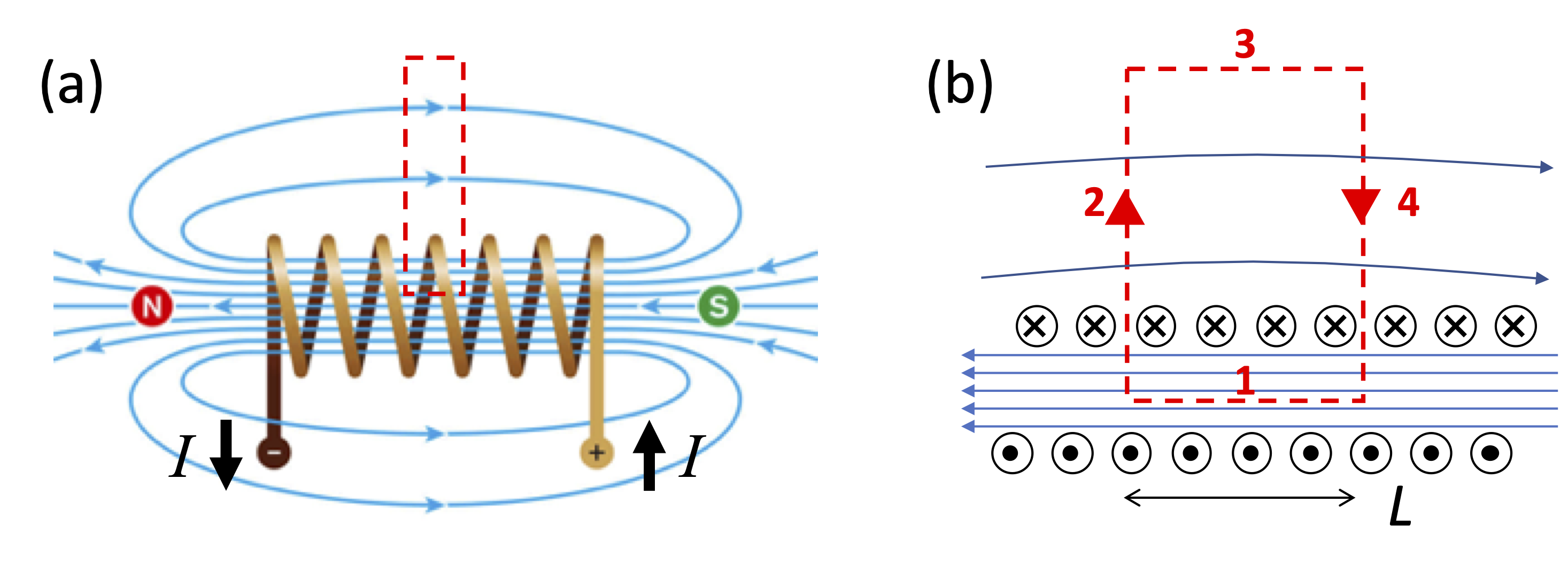
Fig. 12 (a) Field from a solenoid. The Amperian loop used for the calculation is shown by the red dashed line. (b) Expanded version of the Amperian loop.#
Lecture 8:#
Key concepts: Changing the magnetic flux through an area creates an electromotive force. The EMF is given by the Faraday–Lenz Law. The ratio of flux to current is called the inductance.
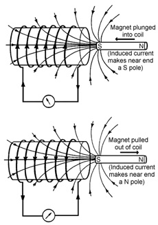
Fig. 13 Electromagnetic induction.#
r6cm
The laws of magnetic induction were discovered by Michael Faraday in 1831–2. The basic experiment consists of a magnet near a coil connected to a galvanometer (a.k.a. a voltmeter), as shown in Fig. 13. When the magnet is stationary, the voltage is zero. Whenever the magnet moves, a voltage is generated. The sign of the voltage depends on the direction in which the magnet is moving. Larger voltages are generated if the magnet is moving faster.
Based on these and similar experiments, Faraday concluded that the electromotive force (EMF) is proportional to the rate of change of the magnetic flux \(\Phi_B\) through the coil. Emil Lenz clarified that the EMF acts to oppose the change that caused it. For example, if you move the magnet closer to the coil, the flux increases. By Lenz’s law, the EMF generates a current that produces a \(B\) field in the opposite direction to the magnet, thereby opposing the increase in the flux. Putting these two insights together, we get the Faraday–Lenz Law (usually just called Faraday’s law) for the EMF \(\mathcal{E}\):
The minus sign follows from Lenz’s law. An important corollary of Faraday’s law is seen by noting that the EMF induced in a wire loop is related to the electric field by
Now the magnetic flux is given by (see eqn (3)):
so that Φ will change if \(\mathbf{B}\) changes with \(t\). A time-varying \(B\)-field generates an EMF by Faraday’s law, and this produces an electric field via eqn (28). We thus conclude that time-varying magnetic fields generate electric fields. This is the origin of Maxwell’s third equation of electromagnetism that will be studied in year 2.
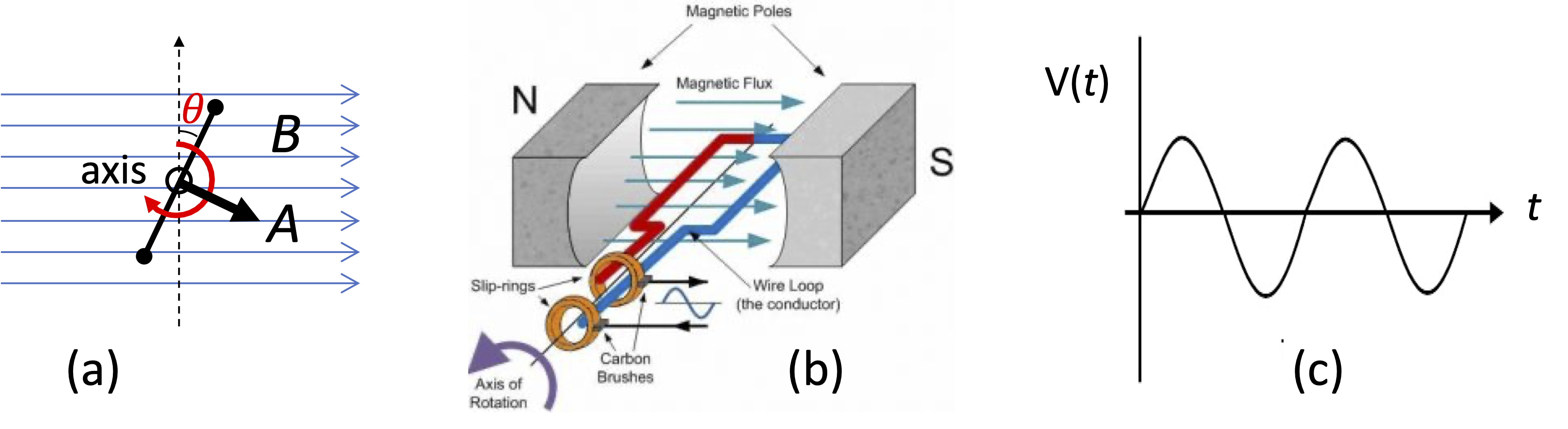
Fig. 14 (a) Coil angled at θ to \(B\)-field. (b) Dynamo. (c) AC voltage output of dynamo.#
The principles of magnetic induction are the basis for alternating current (A.C.) generation in a dynamo. A dynamo is a device that converts mechanical power (specifically: the rotation of a coil) into electricity. To see how this works, consider a wire loop making an angle θ to a magnetic field \(B\), as shown in Fig. 14(a). If the area of the loop is \(A\), then the flux through the loop is given by (see eqn (29)):
If we rotate the loop about its axis with angular velocity ω so that \(\theta(t) = \omega t\) as shown in Fig. 14(b), then we have from Faraday’s law:
We thus generate an AC voltage as shown in Fig. 14(c). The amplitude of the voltage per loop is proportional to the magnetic field, the area, and the rotation rate. By winding many loops together in a coil of \(N\) turns, the voltages in each loop add together, producing a total voltage that increases in proportion to \(N\).
In an electrical power station, mechanical energy is used to turn a turbine inside a large magnet. Coils are attached to the turbine, and this generates AC electricity by Faraday’s law. Cars contain smaller dynamos that generate the electricity that recharges the battery. Since the electrical systems in cars operate on direct current (D.C.), rectifying circuits consisting of diodes and filters must be used to convert the AC that comes out of the dynamo into DC.
Inductors#
We have seen in Lectures 6–7 that current-carrying loops, coils and solenoids generate a magnetic field that is proportional to the current. (See eqns (21) and (26).) Since these have a finite area, the current, \(I\), therefore generates flux through the loop or coil or solenoid that is proportional to \(I\):
The proportionality constant \(L\) that enters here is called the self-inductance, or just inductance for short.
The S.I. unit of inductance is the Henry (symbol: H), which is equivalent to Wb A-1 or T m2 A-1. Like the Farad for capacitance, the Henry is a rather large unit, and typical inductances are in the mH or \(\mu\)H (i.e., microHenry) range.
An electrical component with self-inductance is called an inductor. These are shown as mini-coils in electrical circuits, as in Fig. 15. By Faraday’s law, we see that the EMF generated by an inductor is given by \(\mathcal{E} = -\rm{d}\Phi / {\rm{d} t} = - L \rm{d} I(t) / {\rm{d} t}\). Hence the voltage dropped across an inductor is:
A changing current \(\rm{d} I/\rm{d} t\) will cause a voltage \(V\) that opposes the change in current in the inductor. The faster the change in current, the larger the derivative, and the stronger the voltage that opposes the change in current (especially when \(L\) is also large).
Consider the \(L\)-\(R\) circuit shown in Fig. 15(a). An inductor is connected in series with a resistor and a battery is applied via a switch, S. The switch is closed at time \(t=0\). For time \(t>0\) we have:
where \(V_0\) is the EMF of the battery, and \(I\) is the time-varying current. There are two clear limiting values of \(I(t)\). At \(t=0\) the current must be zero, while at long times after any transients have decayed, we have \(I= V_0/R\). The general solution is
The current thus rises exponentially, with time constant \(L/R\), as shown in Fig. 15(b).
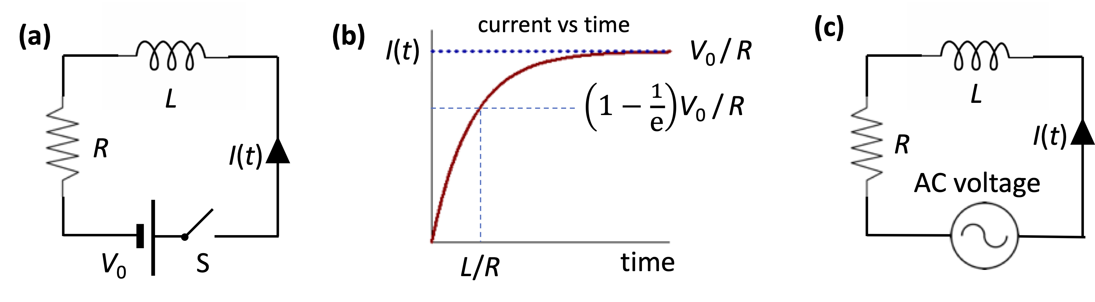
Fig. 15 (a) \(L\)-\(R\) circuit with DC voltage. (b) Time vs current for (a). (c) \(L\)-\(R\) circuit driven by AC voltage.#
Now consider an \(LR\) circuit driven by an AC voltage source, as shown in Fig. 15(c). This will drive an alternating current, written in exponential form as:
where \(I_0\) is the amplitude and ω is the angular frequency. The induced voltage is then calculated from eqn (31) as
By analogy with a resistor, where \(V(t) = I(t) R\), we can write \(V(t) = Z \, I(t)\) for an inductor, where \(Z\) is the impedance. Equation (33) then implies that the impedance of an inductor is given by:
Notice that:
The impedance of an inductor is complex. This is also true for the impedance of a capacitor, where \(Z= 1/{\rm i}\omega C\).
The factor of \({\rm i}\) in the impedance implies that there is a phase lag of \(\pi/2\) radians between the voltage and the current in an inductor, as \({\rm i} = \mathrm{e}^{{\rm i}\pi/2}\).
The impedance increases with frequency. This means that high-frequency alternating currents have a harder time getting through an inductor than low frequency currents.
Lecture 9:#
Key concepts: Atomic dipoles related to orbital motion. Spin dipoles.
In previous lectures we have explored the properties of magnetic dipoles in magnetic field. We shall investigate a bit further into the concept of magnetic dipoles in terms of the atomic structure of the atoms in a magnetic material. We use a very simple model of the atom, in which we have an electron orbiting a nucleus, as shown in Fig. 16. We can think of the orbiting electron as a tiny current loop and work out its magnetic dipole moment as follows. The current is the charge per unit time, which we find from:
where \(-e\) is the charge on the electron, \(r\) is the radius of the orbit, and \(v\) is the speed of the electron. The orbit has area \(A = \pi r^2\), and so the magnetic dipole moment is given by (see eqn (10)):
where \(m_{\rm e}\) is the electron mass.
Now the orbital angular momentum \(L\) of the electron is \(m_{\rm e} vr\), and so we see that \(m = ({-e}/{2m_{\rm e}})L\). In fact, the magnetic dipole moment and angular momentum are both vectors, and so we can write:
where \(\gamma_{\rm e} = -e/2m_{\rm e}\) is the gyromagnetic ratio of the electron, and \(\mu_{\rm B} = e \hbar/2 m_{\rm e}\) is the Bohr magneton. In SI units, the value of \(\mu_{\rm B}\) is \(9.27 \times 10^{-24}\) A m2.
In the Bohr model of the atom, \(L\) is quantised in units of \(\hbar\), with \(L = n \hbar\), where \(n\) is an integer. This implies that the magnetic dipole moment of the atom is quantised in integer units of \(\mu_{\rm B}\). The simplified Bohr-model picture shown in Fig. 16(a) is not compatible with quantum mechanics,
where the value of \(L\) is modified to \(\sqrt{l(l+1)} \hbar\), where \(l = 0, \, 1, \, 2, \cdots\), and the \(z\) component of \(\mathbf{L}\), namely \(L_z\), can take values of \(m_l \hbar\), where \(m_l\) is an integer running from \(-l\) to \(+l\). Nevertheless, the Bohr model is a good start point, and gives us an intuitive idea of the relationship between the atomic magnetic dipole moment and the angular momentum of the electron. It also shows us that the magnitude of atomic dipoles is of order \(\mu_{\rm B}\).
We now consider the spin of the electron, which is an internal degree of freedom, and is analogous to a rotation around its axis. This analogy should not be taken too far, as an electron is, as far as we know, a point particle. The spin \(\mathbf{S}\) of the electron gives it an intrinsic magnetic dipole moment which is additional to any orbital dipole moment it may possess. The spin dipole moment is given by:
where \(g_s = 2.0023193\cdots\) is the electron’s \(g\)-factor. This is very similar to eqn (34), except for the \(g\)-factor. For most practical purposes, \(g_{\rm s}\) is usually taken to be 2. Electrons in atoms in orbits with \(L>0\) possess both orbital and spin angular momentum. Electrons in orbits with \(L=0\) only have spin. Free electrons have a magnetic dipole moment due to their spin.
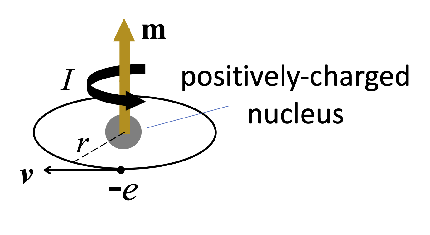
Fig. 16 An atomic dipole. The orbiting electron form a current loop.#
Spin is a quantum-mechanical property of fundamental particles. In general, we can write:
where \(g_i\) is the appropriate \(g\)-factor. The sign of the \(g\) factor usually relates to the charge, which means that it is negative for electron, with \(g_i = - g_{\rm s}\), and \(\mu_i= \mu_{\rm B}\). For protons and neutrons we put \(\mu_i= \mu_{\rm N}\), where \(\mu_{\rm N} =e \hbar/2 m_{\rm N}\) is the nuclear magneton, with \(m_{\rm N}\) being the proton/neutron mass. The value of \(\mu_{\rm N}\) in S.I. units is \(5.05 \times 10^{-27} \, {\rm A \, m}^2\), and so the magnetic dipole moments of protons and neutrons are about 2000 times smaller than that of electrons on account of their larger mass. The \(g\)-factors of protons and neutrons are +5.5857 and -3.8261 respectively. These non-integer values point to the fact that protons and neutrons are actually composite rather than elementary particles. The negative, non-zero value for the neutron is particularly striking, given that the neutron is uncharged.
Let us consider the path of an uncharged particle (e.g. a neutron) through a magnet with a non-uniform field.
Particles with non-zero magnetic dipole moments will experience a force according to eqns (14) and (36):
where \(S_z\) is the \(z\)-component of the spin. Therefore, given a magnetic field, the particle experiences a force along the \(z\)-direction that is directly proportional to its spin.
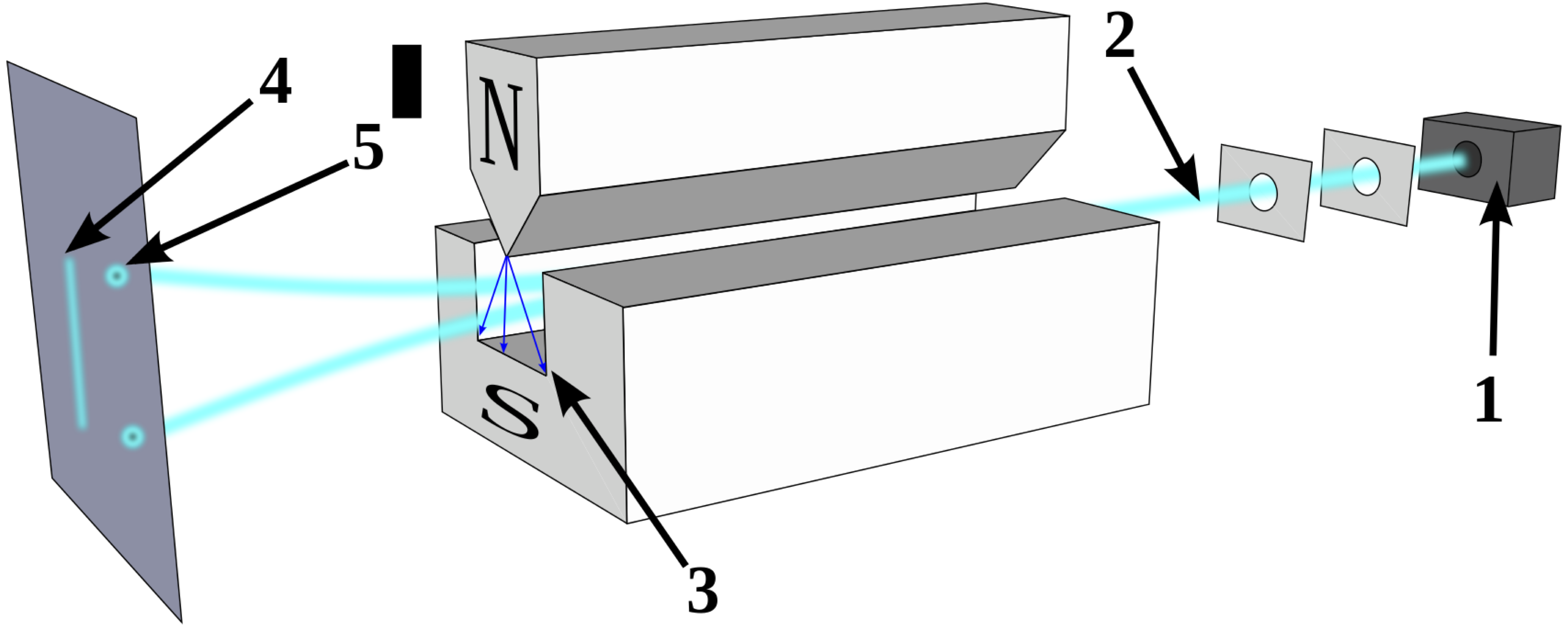
Fig. 17 The Stern–Gerlach experiment. Note the non-uniform magnetic field in the vertical direction that is created by the shape of the magnets. 1: Particle source. 2: Particle beam. 3: Region with non-uniform \(B\)-field. 4: Result expected for classical particles with continuous values of \(m_z\). 5: Result obtained for spin 1/2 particles.#
This phenomenon is demonstrated in a Stern-Gerlach experiment (see figure 17). Particles are sent from a source to a fluorescent screen. A bright dot will appear at the position where the particle hits the screen. In the absence of the magnetic field, the particles travel along a central axis connecting the source with the screen. When the magnetic field is present, we would expect a continuous fluorescent line spanning the possible values of the \(z\)-components of the spin, \(S_z\).
Instead, the dots will appear in two regions: one slightly up from the central axis, and one slightly down from the axis, as shown in figure 17. This means that \(S_z\) can take only two values. When we work out these values from the magnetic field gradient and the positions of the dots on the screen, we find that
We thus have “spin up” and “spin down” particles with \(S_z/\hbar = \pm1/2\), i.e. “spin 1/2” particles.
Electrons, protons and neutron are examples of such spin 1/2 particles. In the case of electrons with \(|g|\approx 2\), we have \(m_z = \pm \mu_{\rm B}\). The spin of the electron is extremely important for understanding the properties of magnetic materials such as iron.
Lecture 10:#
Key concepts: The magnetic susceptibility determines how materials respond to fields, and whether they retain magnetisation after an external field is turned off.
We have seen in the previous lecture that the atoms that make up a material can have a magnetic dipole moment. The magnetic dipoles \(\mathbf{m}\) inside a material collectively generate a magnetization, \(\mathbf{M}\), which is defined as the magnetic dipole moment per unit volume. The magnetization is a vector and is worked out from the vector sum of all the magnetic dipoles inside the material. We can thus write \(\mathbf{M} = N \langle \mathbf{m}\rangle\), where \(N\) is the number of magnetic atoms per unit volume, and \(\langle \mathbf{m}\rangle\) is the average of the vector sum of all atomic dipoles pointing in the same direction. The units of magnetization are A m-1. Notice that Ampre’s law (eqn (22)) implies that \(B * {\rm m} = \mu_0 * {\rm A}\). Hence \(\mu_0 \mathbf{M} \equiv \mu_0 * {\rm A\,m}^{-1}\) has the dimensions of magnetic field, and we can find the magnetic field inside a magnetic material by adding the field due to the magnetization to the applied external field \(\mathbf{B}_0\):
With the exception of ferromagnetic materials that will be discussed below, we expect a material to be magnetized only when an external field is applied, and that the magnitude of the magnetization will be proportional to the field. We can thus write:
where \(\chi_{\rm m}\) is the dimensionless magnetic susceptibility of the material. On substituting into eqn (37), we find:
This allows us to define the relative magnetic permeability \(\mu_{\rm r}\) as:
which implies that the field inside the magnetic material is given by
\(\mu_{\rm r}\) gives the magnetic permeability of a material compared to the vacuum.
The magnetic properties of a material are classified by the sign and magnitude of \(\chi_{\rm m}\), or, equivalently, of \((\mu_{\rm r}-1)\). This leads to three broad classes of behaviour, which are summarized in Table 2 and are discussed separately below.
Diamagnetism#
Diamagnetism is observed in materials that are non-magnetic. These are materials that are composed of molecules with zero magnetic dipole moment. The vast majority of materials fall into this class, as chemistry makes compounds with filled atomic shells, and filled atomic shells have no magnetic dipole moment. This is because chemical bonds work by pairing off spin up and spin down electrons, giving no net spin (or orbital magnetic moments) for the whole molecule.
The magnetic susceptibility \(\chi_{\rm m}\) of diamagnetic materials is small and negative.
It is approximately independent of temperature. The negative sign can be considered to be a consequence of Lenz’s law, which requires that the applied field induces microscopic effects that oppose the field that is applied.
\(\chi_{\rm m}\) |
\(|\chi_{\rm m}|\) |
Comments |
|
Diamagnetic |
negative |
small |
Individual molecules have zero dipole moment |
Paramagnetic |
positive |
small |
\(\chi_{\rm m} \propto 1/T\) |
Ferromagnetic |
positive |
large |
Can be magnetized even with \(\mathbf{B}_0 = 0\) |
Paramagnetism#
Paramagnetic materials contain molecules with a non-zero dipole moment \(\mathbf{m}\). This requires unfilled atomic shells, and so is mainly restricted to compounds that contain transition metal or rare-earth elements (also called lanthanides), which have unfilled “d” and “f” shells, respectively, even after forming compounds.
The microscopic dipoles in a paramagnet do not interact with each other, and point in random directions at \(B=0\), giving no magnetization. When an external field is applied, the dipoles tend to align along the field, producing a net magnetization parallel to \(\mathbf{B}\), implying that \(\chi_{\rm m}\) is positive. The tendency to align with \(\mathbf{B}\) follows from eqn (13), namely \(U=-\mathbf{m}\cdot \mathbf{B}\), which means that the state with \(\mathbf{m}\) parallel to \(\mathbf{B}\) is lower in energy by \(2 mB\) compared to the state with \(\mathbf{m}\) antiparallel to \(\mathbf{B}\). The average dipole moment per molecule \(\langle \mathbf{m}\rangle\) is then determined by the competition between the tendency to align along the field and the random thermal motion. At room temperature, the magnetic interaction energy \(2m B\) (with \(m \sim \mu_{\rm B}\)) is much smaller than the thermal energy \(k_{\rm B}T\) at reasonable laboratory fields, and so the amount of alignment is only small, explaining why \(\chi_{\rm m}\) is small. The susceptibility increases at low temperatures, since there is less random thermal motion. Experiments (and calculations from statistical mechanics done in Year 2) show that \(\chi_{\rm m} \propto 1/T\). This is called Curie’s law.
At very large field strengths, all the dipoles are aligned, and we will have \(\mathbf{M} = N \mathbf{m}\), where \(N\) is the number of molecules per unit volume. This is the largest value of \(|\mathbf{M}|\) that the material can have, and is called the saturation magnetization. The field required to saturate a paramagnet at room temperature is huge, and so the saturated magnetization is only observed at low temperatures.
Ferromagnetism#
The magnetic susceptibility of a ferromagnetic material is large and positive. This gives large values of the relative magnetic permeability \(\mu_{\rm r}\), typically -. In a ferromagnetic material, the magnetic dipoles of the atoms interact strongly and spontaneously align parallel to each other.
They can therefore have magnetization even at zero external fields, which is the basis for permanent magnets. Examples are iron (ferrum in latin), cobalt and nickel.
Ferromagnetic materials contain domains in which all the atomic dipoles are aligned. The domains, however, are not necessarily aligned parallel to each other, and this is why a ferromagnet can be unmagnetized, even though all the dipoles are aligned parallel to each other at a microscopic level. The application of an external field shifts the domain boundaries or causes whole domains to flip, as shown in Fig. 18(a). The size of the domains pointing along the field increases, and the material acquires a net magnetization. It takes energy to move the domain boundary, and so the domain sizes do not change much after the external field is removed. Hence there is a net magnetization at \(B_0 = 0\), although it will not be equal to \(Nm\), where \(N\) is the number of atoms and \(m\) is the atomic dipole moment, as some of the domains are pointing in opposite directions.
The magnetization curve (i.e. a graph of \(M\) against applied field) of a ferromagnetic material exhibits hysteresis, shown in figure 18(b). Once magnetized in a strong \(\mathbf{B}\) field, the domains remain predominantly pointing along the same direction, giving a remanent magnetization at \(B_0 = 0\). The magnetization can only be removed by applying a large field in the opposite direction (or by heating the sample above its critical temperature). The field required to switch the direction of the magnetization is called the coercive field.
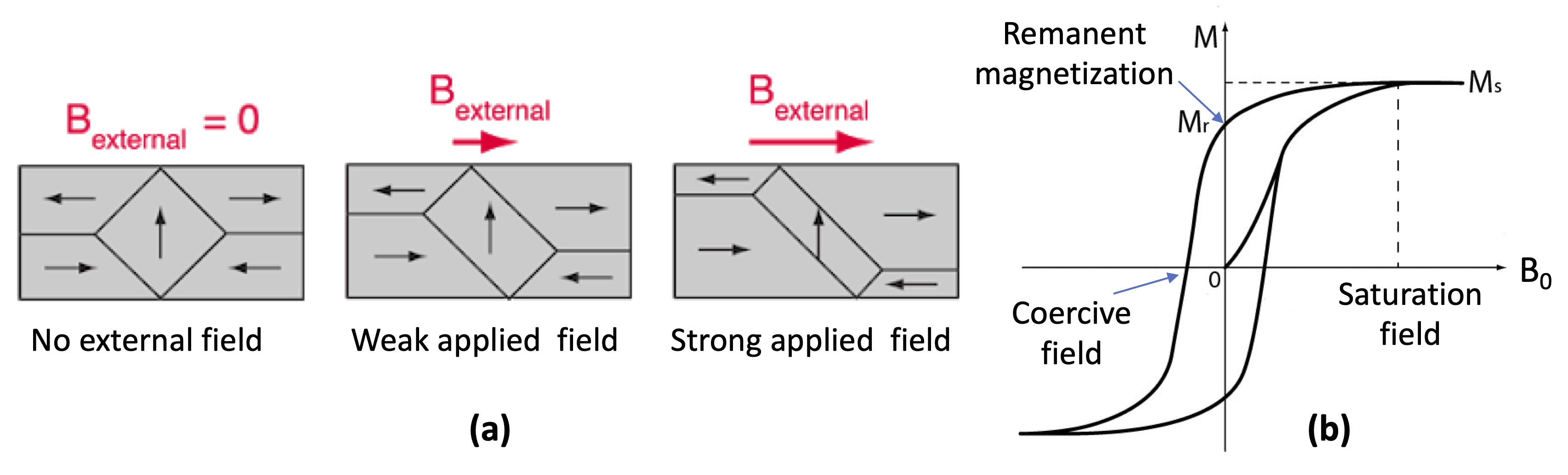
Fig. 18 (a) Growth of magnetic domains as \(\mathbf{B}\) increases. The initial state is unmagnetized, and the size of the domains pointing parallel to the external field increase as \(\mathbf{B}\) increases. When the external field is removed, the domain sizes remain largely unchanged, giving net magnetization at \(\mathbf{B}_0=0\). A large field in the opposite direction must be applied to switch the magnetization to the opposite direction by making the domain sizes change. (b) Hysteresis loop, starting from an unmagnetized sample with \(M=0\).#
The \(\mathbf{H}\) field#
When we apply a magnetic field to a material, we have two fields to consider: the external field and the net field that includes the magnetization of the material. A similar situation arises with electric fields applied to dielectric materials. We have the external field \(\mathbf{E}\) that creates a polarization \(\mathbf{P}\), leading to the concept of the displacement field \(\mathbf{D}\) defined by:
where χ is the electric susceptibility defined by \(\mathbf{P} = \epsilon_0 \chi \mathbf{E}\), and \(\epsilon_{\rm r}=(1+\chi)\) is the relative permittivity of the material. It is clear here that \(\mathbf{E}\) is the fundamental field, and \(\mathbf{D}\) is a derived field that includes the response of the dielectric.
The situation with magnetic fields is not so tidy. In analogy with electricity, we define two fields: \(\mathbf{B}\) and \(\mathbf{H}\). Old textbooks consider \(\mathbf{H}\) to be the fundamental field, and \(\mathbf{B}\) the derived one that includes the response of the material. We then write: The \(\mathbf{H}\) field is confusingly also called the magnetic field, and \(\mathbf{B}\) is then called the magnetic induction or magnetic flux density.
In S.I. units we now say that \(\mathbf{B}\) is the fundamental field, and \(\mathbf{H}\) is a derived one that includes the response of the material. We add a subscript on \(\mathbf{B}\) to identify the applied field \(\mathbf{B}_0\), and define \(\mathbf{H}\) as:
where \(\mathbf{B}\) is the magnetic field inside the material defined in eqn (40). On combining this, for example, with eqn (37), we then find \(\mathbf{B}_0 = \mu_0 \mathbf{H}\), which makes the link between \(\mathbf{H}\) and the fundamental field apparent.
Lecture 11:#
Key concepts: energy is stored in a magnetic field; the energy in an LC circuit oscillates back and forth between the electric and magnetic fields, whereas the energy in a travelling electromagnetic wave is shared equally by the two fields.
The easiest way to start thinking about the energy in magnetic fields is to work out the energy stored in an inductor. Consider again the \(LR\) circuit shown in Fig. 15 covered in Lecture 8. When the switch is closed, the current increases until it reaches its final value of \(I_0 = V_0/R\). (See eqn (32).) At any instant, the voltage across the inductor is \(V(t)=L {\rm{d} I}/{\rm{d} t}\) (see eqn (31)), where \(I\) is the current at time \(t\). Lenz’s law tells us that this opposes the current, and so power must be applied to drive the current. This power is given by:
The work done to establish the current is found by integrating \(P(t)\):
We thus conclude that the energy stored in an inductor carrying a current \(I\) is given by:
This energy is stored in the magnetic field. To see this, consider an air-cored solenoid of area \(A\) and length \(l\), with \(n\) turns per unit length. The flux through each turn is \(BA\), and so the total flux is \(\Phi = BA N\), where \(N=nl\) is the total number of turns. With \(B= \mu_0 n I\) from eqn (26), this implies that the inductance defined in eqn (30) is \(L = \Phi/I = \mu_0 n^2 A l\). The inductor energy is then given by:
Now the volume of the solenoid core is \(\mathcal{V} = Al\), and so we see that the energy density \(u_B\) is:
This is a general result that applies to all cases, not just the solenoid. Note that we use the lower case to distinguish the energy per unit volume, \(u_B\), from the total energy, \(U\).
If the core has relative permeability \(\mu_{\rm r}\), the field in the core increases to \(\mu_{\rm r}B_0\), where \(B_0= \mu_0 n I\). This implies that both the flux and the inductance increase by \(\mu_{\rm r}\), and so we get:
and hence, using \(\mu = \mu_{\rm r} \mu_0\) for the total magnetic permeability:
LC circuits#
Consider the \(LC\) circuit shown in Fig. 19(a) in which a capacitor is connected to an inductor via a switch, S, and to a battery with an EMF of \(V_0\) via switch S\('\). The capacitor is charged up with S\('\) closed and S open. The battery is then disconnected by opening S\('\), leaving a charge \(Q_0=CV_0\) on the capacitor. Switch \(S\) is then closed at time \(t=0\) so that the capacitor can discharge into the inductor, giving a time-varying charge \(Q(t)\) on the capacitor and a time-varying current \(I(t)\) in the circuit.
We can analyse the \(LC\) circuit for time \(t>0\) by noting that the total voltage drop around a closed circuit loop must be zero (Kirchhoff’s second circuit law):
The two terms represent the voltages dropped across the capacitor and inductor respectively. (See eqn (31).) On substituting \(I = \rm{d} Q/ \rm{d} t\) and rearranging, this becomes:
We can compare this to the equation of motion of an undamped simple harmonic oscillator. For example, for a mass \(m\) on a spring with spring constant \(k\), we have
where \(\omega = \sqrt{k/m}\). The solution is
where ϕ is a phase factor determined by the starting conditions. This makes it apparent that eqn (44) describes oscillations in which the charge on the capacitor varies sinusoidally with time:
where the angular frequency ω of the oscillations is given by:
We can find \(I(t)\) by differentiating with respect to time:
At \(t = 0\), \(Q\) is at it maximum value of \(C V_0\), and so we can put \(Q_0 =CV_0\) and \(\phi = \pi/2\). The solution for \(Q(t)\) and \(I(t)\) is then:
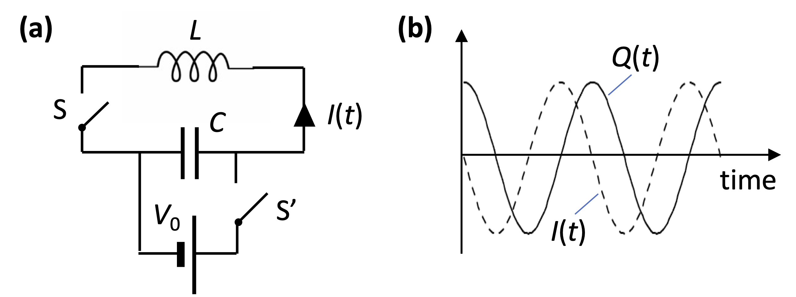
Fig. 19 (a) An \(LC\) circuit. The capacitor is charged by closing switch S\('\) with switch S open. Oscillation occurs when the battery is disconnected and switch S is closed. (b) Time dependence of the charge on the capacitor and the current flowing in the circuit.#
The oscillating charge and current are plotted against time in Fig. 19(b). The capacitor discharges, generating a time-varying current through the inductor that induces a voltage to recharge the capacitor to \(Q=-CV_0\). The process then repeats itself, with the current flowing in the opposite direction. These oscillations are the basis for electronic oscillators that generate AC signals. The frequency of the oscillations is given by eqn (46) and can be tuned by varying either \(L\) or \(C\). In practice, it is usually easier to vary \(C\), and this is the basis for tuned circuits, as used, for example, in radio receivers.
The charging and discharging of the capacitor in an oscillating \(LC\) circuit raises a question about energy conservation. A charged capacitor stores energy given by
while an inductor stores energy given by eqn (41):
The time variation of the energies in the \(LC\) circuit can be worked out by substituting \(Q(t)\) and \(I(t)\) into eqns (48) and (49), giving, respectively:
On noting from eqn (46) that \(\omega^2 = 1/LC\), we see that \(U_L = \frac{1}{2} C V_0^2 \sin^2 {\omega t}\), and hence that the total energy is constant: The total energy in the LC circuit is thus constant and oscillates back and forth between the capacitor and the inductor. The energy is initially stored in the \(E\) field of the capacitor. As the capacitor discharges, the current increases, generating a \(B\) field in the inductor. Hence the energy oscillates between the \(E\) field in the capacitor and the \(B\) field in the inductor, which have a \(90^\circ\) phase shift between them.
Energy in electromagnetic waves#
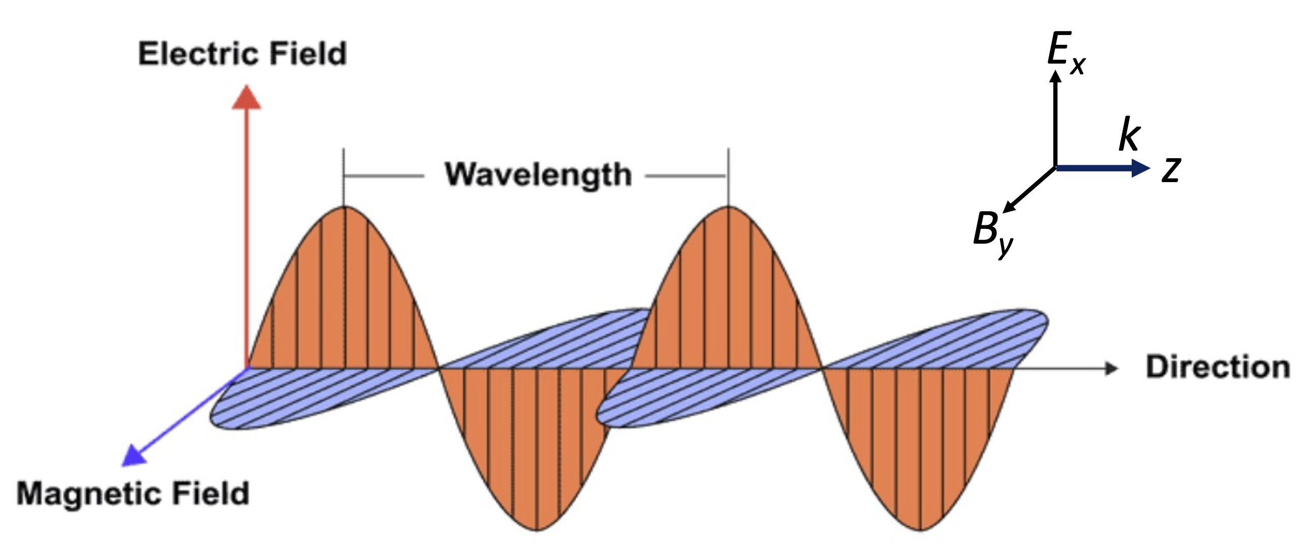
Fig. 20 Oscillating fields in an electromagnetic wave.#
Electromagnetic (EM) waves travelling through a vacuum consist of oscillating electric and magnetic fields. The fields are at right angles to each other, and to the direction of propagation. For example, for a wave propagating in the \(+z\) direction, we could have fields given by:
where \(\omega = ck\), \(c\) being the velocity of light. The relative directions of the fields and \(\mathbf{k}\)-vector are shown in Fig. 20. Note that \(\mathbf{E}\), \(\mathbf{B}\) and \(\mathbf{k}\) form a right-handed system.
A full understanding of how the laws of electromagnetism explain EM waves requires solution of Maxwells’ equations, which will be done in Year 2. It can be shown that the amplitudes of the electric and magnetic fields are related to each other by
This allows us to reach a very important conclusion about the energy density in the EM wave. Since there are two types of field, the total energy density is given by:
where \(u_E\) and \(u_B\) are the energy densities of the electric and magnetic fields, respectively. We know from electrostatics that \(u_E = \epsilon_0 \mathbf{E} \cdot \mathbf{E} /2\), and we have worked out \(u_B\) in eqn (42). We thus find, using eqn (51), that:
Now it can be shown from Maxwell’s equations that \(c^2 = 1/\epsilon_0 \mu_0\), which implies that the first and second terms in eqn (52) are the same. We thus conclude that the energy densities of the electric and magnetic fields in an EM wave are identical.
There is an interesting difference here between the travelling EM wave and the \(LC\) circuit considered previously. In the \(LC\) circuit, the electric and magnetic fields are out of phase and the energy oscillates back and forth between them. By contrast, in a travelling EM wave, the oscillating \(E\) and \(B\) fields are in phase, and the energy is split equally between them. This is a consequence of the fact that the \(LC\) circuit can be considered as standing EM wave, where the two travelling wave components propagating in opposite directions interfere to make the energy oscillate between the fields.
An appendix on vectors#
Let us consider the vector \(\mathbf{a}\), where
This is a vector with component \(a_x\) along the \(x\) axis, \(a_y\) along the \(y\) axis, and \(a_z\) along the \(z\) axis. It is convenient to write this either as a \((3 \times 1)\) column matrix:
or as a \((1 \times 3)\) row matrix:
The length of this vector is:
We can form a unit vector pointing in the direction of \(\mathbf{a}\) by dividing \(\mathbf{a}\) by its length:
Note that the ‘hat’ symbol on \(\hat{\mathbf{a}}\) indicates that it is a unit vector, just like the hat symbols on \(\hat{\mathbf{i}}\), \(\hat{\mathbf{j}}\) and \(\hat{\mathbf{k}}\).
The scalar product of two vector \(\mathbf{a}\) and \(\mathbf{b}\) (also called the “dot” product) is given by:
By writing this in column vector format, we see that we just multiply the rows and add:
This works out to be:
where θ is the angle between \(\mathbf{a}\) and \(\mathbf{b}\). A convenient way to work out \(\mathbf{a} \cdot \mathbf{b}\) is by using the product of the row and column vectors:
Note that
and that \(\mathbf{a} \cdot \mathbf{b} = 0\) when \(\mathbf{a}\) and \(\mathbf{b}\) are orthogonal (i.e. the angle between them is \(90^\circ\)).
The vector product (or “cross” product) of two vectors is written:
The vector \(\mathbf{c}\) points in the direction which is orthogonal to both \(\mathbf{a}\) and \(\mathbf{b}\), and has length:
where θ is the angle between \(\mathbf{a}\) and \(\mathbf{b}\). Note that \(\mathbf{a} \times \mathbf{b} = 0\) when \(\mathbf{a}\) and \(\mathbf{b}\) are parallel.
The direction of \(\mathbf{a} \times \mathbf{b}\) is found from the right-hand rule, as shown in Fig. 21. Point the first finger of your right-hand along \(\mathbf{a}\), your second finger along \(\mathbf{b}\), and your thumb gives the direction of \(\mathbf{a} \times \mathbf{b}\). Alternatively, imagine the plane that contains the vectors \(\mathbf{a}\) and \(\mathbf{b}\), and \(\mathbf{a} \times \mathbf{b}\) is in the normal direction (i.e. perpendicular) to the plane. Your thumb gives the direction of \(\mathbf{a} \times \mathbf{b}\) when curling the fingers of your right hand from \(\mathbf{a}\) to \(\mathbf{b}\).
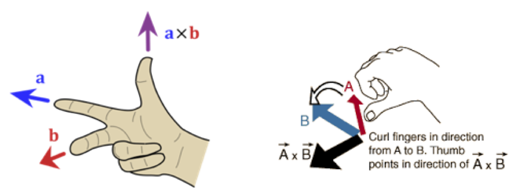
Fig. 21 Right-hand rules for vector products#
We can work out the components of \(\mathbf{a} \times \mathbf{b}\) from the determinant: This can be written
You remember this as follows. To get the component in row \(i\), cross out row \(i\) in the column vectors of \(\mathbf{a}\) and \(\mathbf{b}\), and then take the determinant of what is left, remembering to add a \(-\) sign for the middle row.