
Chapter 1: Introduction#
This module combines elements of two now retired second year models PHY217 (Observational Astronomy, precursor to PHY241) and PHY232 (Interstellar Medium) namely spectrographs, interstellar medium and nebulae.
These lecture notes were created for the 2023/24 session, as part of a refresh of the module content in order to connect introductory material from PHY104 (Introduction to Astrophysics) to more advanced radiative transfer content in PHY305 (Stellar Atmospheres). Radiative transfer is now deferred to third year (parallel-ray radiative transfer topics will not be examined in PHY242), while an expanded treatment of data reduction, atomic physics and interstellar extinction is provided.
Observations of astronomical objects across much of the electromagnetic spectrum involve either imaging (covered extensively in PHY241) or spectroscopy. Interpretation of the latter requires knowledge of atomic physics which usually come from laboratory studies or theoretical developments linked to quantum mechanics. In this introduction I shall describe some of the major advances that astronomical spectroscopy has been fundamental in establishing, starting with a recap on material from PHY104.
Historical recap of stellar spectroscopy#
Although Isaac Newton was the first to recognise that the Solar spectrum is made up of coloured light with his double prism experiment in 1672, developments by Joseph von Fraunhofer (1787-1826) - including the first use of diffraction gratings in 1821 as well as prisms - permitted him to catalogue hundreds of absorption lines in the Solar spectrum, the strongest of which (e.g. Fraunhofer D line) remain in common use today. Prominent lines in the Solar spectrum are indicated in Fig. 1.
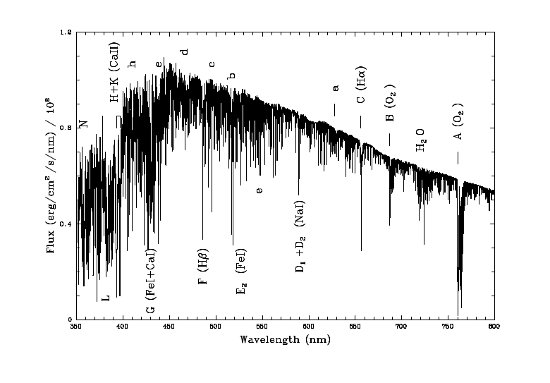
Fig. 1 Solar spectrum (Kurucz et al. 1984) including Fraunhofer lines identified (adapted from Fig 12.2 of Mark Fox’s Atomic Physics textbook.#
The first step towards understanding Fraunhofer’s observations were provided by experiments of Gustav Kirchhoff (1824-1887) and Robert Bunsen (1811-1899) who established in 1860 that the colour of light emitted by burning metals gave an exact match to the wavelength of some Fraunhofer lines, as Kirchhoff wrote in 1862:
The dark D lines in the solar spectrum allow one therefore to conclude that sodium is present in the solar atmosphere
These experiments demonstrated that the Fraunhofer lines were a direct consequence of the atomic composition of the Sun.
In addition, Kirchhoff & Bunsen’s experiments established a series of rules for the type of spectrum observed from various types of light sources (Fig. 2). The found that hot, low density gases produced a series of emission lines, characteristic to the composition of the gas, reminiscent of nebulae that William Huggins (1824-1910) observed in the 1860s. They also found that when dense gas was observed through a cooler, lower density gas, the spectrum observed was a continuous spectrum in which a series of absorption lines superimposed, reminiscent of the Solar spectrum.
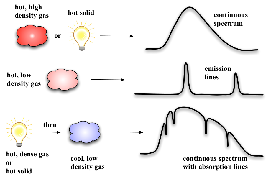
Fig. 2 Kirchhoff & Bunsen’s empirical rules for the type of spectrum observed from different types of light sources.#
The introduction of objective prism spectroscopy in the late 1800s and societal changes permitted the Harvard College Observatory group, led by William Pickering and a large team of predominantly female team of (human) computers to devise the modern classification of stellar spectra, arranging stars into seven spectral classes, OBAFGKM, according to absorption strengths of different elements, in which A-type stars possess the strongest hydrogen lines, followed by B-type. Williamina Fleming (1857-1911), Antonia Maury (1866-1952) and Annie Cannon (1863-1941) led the classification of several hundred thousand stars, although the physical meaning of their spectral line properties awaited future developments in the early 20th century.
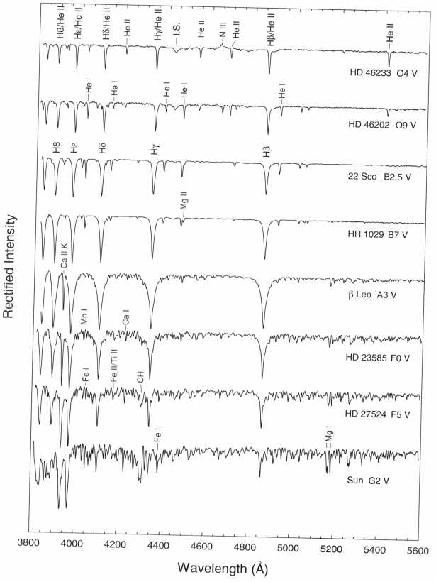
Fig. 3 Main sequence stars from G2 V to O4 V from Fig 2.2 of Gray & Corbally’s Stellar Spectral Classification. These spectra have a resolution of 3.6Å, and have been offset by 0.7 continuum units for clarity.#
In particular, an understanding of atomic structure (Ernest Rutherford, Niels Bohr) plus electron excitation conditions courtesy of Ludwig Boltzmann,
where relative populations \(N\) involve statistical weights \(g\), helped to explain the observed spectral features. In addition, ionization conditions courtesy of Meghnan Saha’s extension of the Boltzmann equation to ionization stages,
where relative populations of adjacent ionization stages \(N\) involve partition functions \(Z\). Here \(\chi_{\rm ion}\) is the ionization energy and \(n_{e}\) is the electron density. These provided the tools with which physical properties and chemical abundances of stars could be determined. This was first undertaken by Cecilia Payne (1900-1979) whose doctoral dissertation in 1925 for the first time concluded that hydrogen is by far the most abundant element in stars.
Modern classification of stars involves a second criteria beyond spectral class, namely luminosity class, which is obtained from the detailed appearance of spectral lines, usually optical hydrogen (Balmer) lines. This (MKK) system was devised by William Morgan, Philip Keenan and Edith Kellman in 1943. Most stars are (hydrogen burning) main sequence stars known as dwarfs (luminosity class V), with high surface gravities. Fig. 3 shows examples of main sequence stars from G2 V to O4 V. The next most common type of star observed are giants (luminosity class III) which are post-main sequence evolved stars, with lower surface gravities. High luminosity evolved stars are supergiants (luminosity class I) possessing still lower surface gravities.
You will have to wait until PHY305 (Stellar Atmospheres) to find out how detailed physical properties and elemental abundances can be obtained from stellar spectroscopy, but you will get to learn how abundances can be determined from spectroscopy of gaseous nebulae.
Doppler shifts#
Spectroscopy also provides information on radial motion of astronomical objects, through Doppler shifts, named after Christian Doppler (1803-1853). For non-relativistic motions, radial velocities \(v_r\) can be obtained from the measured wavelength shift (\(\Delta \lambda = \lambda_{\rm obs} -\lambda_0\)) relative to the laboratory rest wavelength \(\lambda_0\) via
Spectroscopic monitoring, via measured Doppler shifts permit reliable mass determinations of stars in binaries (double-lined eclipsing binaries), plus mass estimates of exoplanets orbiting their parent stars, and the nature of compact objects, most famously Cygnus X-1 for which Louise Webster and Paul Murdin provided the first indirect evidence of a stellar mass black hole in 1972.
Doppler shifts also permitted Edwin Hubble (1889-1953) to combine the relationship between period and brightness of Cepheid variables (Leavitt law, named after Henrietta Leavitt who made the discovery in 1908) in nearby galaxies with measured radial velocity measurements. The resulting Hubble law, which relates the distance of an object (\(d\)) and its redshift \(z (= \Delta \lambda/\lambda_0\)) via
where \(H_0\) is the present value of the Hubble constant (\(\sim\)70 km s-1 Mpc-1). This was published in 1929 and empirically established the expansion of the universe. This result has been predicted by Alexander Friedmann in 1922 based on Einstein’s General Relativity, and also anticipated by Georges Lemaître who had independently developed a model for an expanding universe in 1927 that was consistent with the observed receding velocities of galaxies, such that the Hubble law is more correctly described as the Hubble-Lemaître law.
For very distant objects in the universe (\(z \geq 0.1\)), Special Relativity needs to be taken into account, such that the relativistic Doppler formula is
The advent of large ground based (e.g. Keck, VLT) and space-based (Hubble, James Webb) has permitted the discovery of very distant star-forming galaxies, active galaxies and stellar explosions (supernovae, gamma-ray bursts) via the Doppler shift technique.
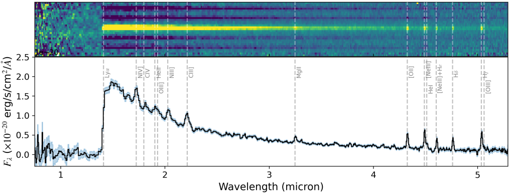
Fig. 4 JWST-NIRSpec observations of the extremely high redshift galaxy GN-z11 (Bunker et al. 2023)#
For example, GN-z11 was first identified in 2016 as a \(z\sim11\) galaxy from identification of Lyman-α emission in Hubble Space Telescope slitless grism spectroscopy. Recent JWST spectroscopy with the NIRSpec instrument is shown in Fig. 4 and confirms its high redshift such that its rest frame ultraviolet spectrum is (red)shifted into the near-infrared part of the spectrum, and its rest frame optical spectrum is (red)shifted into the mid-infrared part of the spectrum. GN-z11 represents a bright star-forming galaxy only 430 Myr after the Big Bang.
Spectral resolution#
In PHY241 you will have learnt about the importance of spatial resolution in astronomical imaging, such that the highest resolving power (θ in radians) of a telescope is described via the diffraction limit of the Rayleigh criterion,
where λ is the wavelength of observation and \(D\) is the telescope diameter, and equates to
recalling that there are 206,265 arcsec in a radian. Fig. 5 compares mid-infrared imaging of a region of the Large Magellanic Cloud obtained with Spitzer (\(D\)=0.85m) and JWST (\(D\)=6.5m) illustrating the dramatic difference in impact quality.
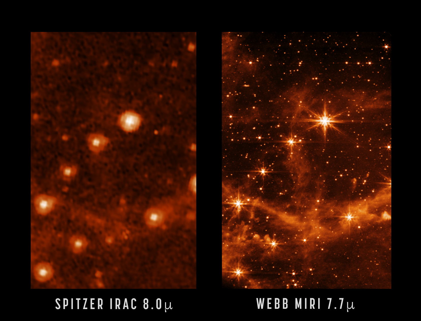
Fig. 5 Comparison between mid-IR imaging of a region of the Large Magellanic Cloud (LMC) with Spitzer (\(D\)=0.85m) and JWST (\(D\)=6.5m). Credit: NASA/JPL-Caltech (left), NASA/ESA/CSA/STScI (right).#
Spectrographs operating at X-ray, ultraviolet, optical and infrared wavelengths require one, or more, methods of dispersing the light, namely prisms, diffraction gratings or grating prisms (grisms). The resolving power, \(R\), a fundamental characteristic of astronomical datasets, is defined as
for observations at λ and \(\lambda + \Delta \lambda\) is the closest wavelength to λ that can be separated. Recall from Eqn (3) that \(R\) is the reciprocal of the Doppler shift, so the value of \(R\) describes the ability of a spectrograph to detect such shifts, i.e. unless the Doppler shift is larger than a resolved spectral element, it would not be detected.
In general, the physical information that can be deduced from spectra increases with the resolution. Let us first consider the resolving power of broad-band imaging. The Johnson V-band filter has a central wavelength of \(\lambda_0\) = 5500Å, and a bandwidth of \(\Delta \lambda \sim\) 1000Å, so \(R \sim 5.5\).
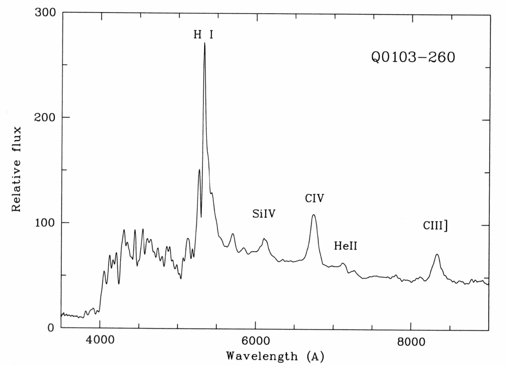
Fig. 6 Low resolution (\(R\sim350\)) spectroscopy of the high redshift quasar Q0103-260 obtained with the FORS1 instrument at VLT using the 150I grism (Dietrich et al. 1999).#
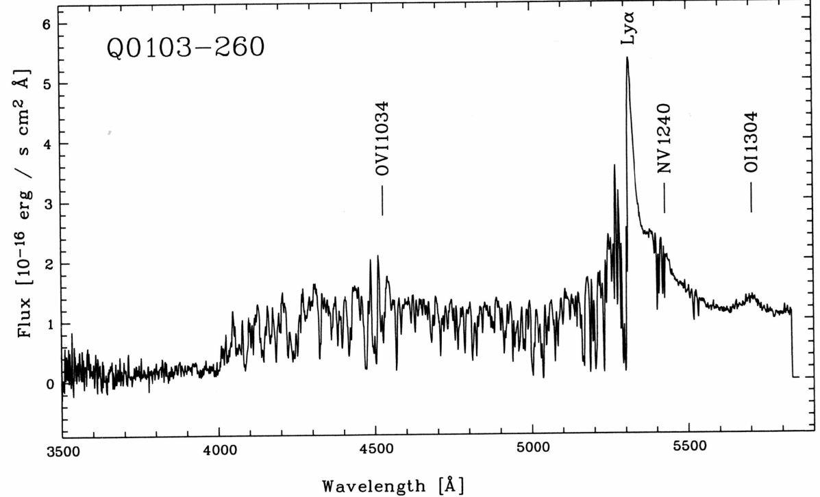
Fig. 7 Medium resolution (\(R\sim2000\)) spectroscopy of the high redshift quasar Q0103-260 obtained with the FORS1 instrument at VLT using the 600B grism (Dietrich et al. 1999).#
We will describe the origin of Eqn. (5) in the next Chapter, but for the moment let us consider low, medium and high resolution spectroscopic observations. We will use the same object, the ‘bright’ (\(m_{v} \sim 18.8\) mag) quasar Q0103-260 at \(z\) = 3.365, to illustrate these different resolving powers.
The low resolution (\(R \sim 350\)) spectrum (Fig. 6), obtained with the (recently retired) FORS1 instrument at the VLT in Chile shows sufficient details to identify the object unambiguously as a high-redshift quasar, with the redshift measurable from various broad emission lines of hydrogen, helium, carbon, oxygen and silicon. The spectrum also indicates the presence of continuum absorption shortward of 4000Å, evidence for line absorption shortward of 5300Å, but none of the (weak) absorption lines can be identified. One advantage of low resolution spectroscopy is that the entire optical spectrum can be recorded with a modern CCD detector.
The medium resolution (\(R \sim 2000\)) spectrum (Fig. 7) was obtained with the same FORS spectrometer, albeit a different grating (more on this later), but is now able to resolve the features below 5300Å into a large number of narrow absorption lines, plus a few more at longer wavelengths that were not apparent in the low resolution spectrum (Dietrich et al. 1999 describe these observations).
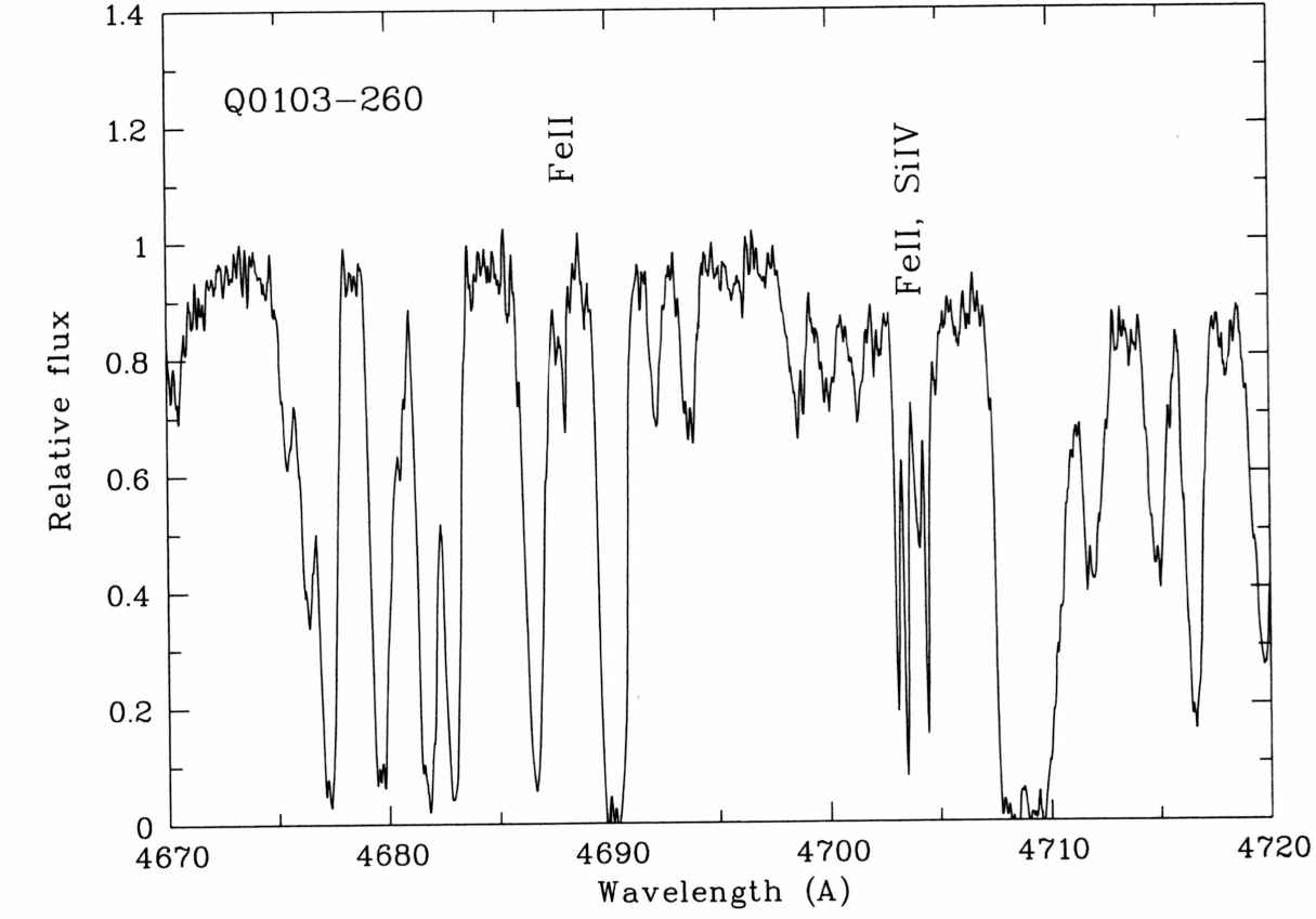
Fig. 8 High resolution (\(R\sim40,000\)) spectroscopy of the high redshift quasar Q0103-260 obtained with the UVES instrument at VLT (Frank et al. 2003).#
These lines are fully resolved in the small section (50Å) of a high resolution (\(R \sim 40,000\) spectrum of Q0103-260 obtained with the UVES echelle spectrograph also at the VLT (Fig. 8 Frank et al. 2003). Most of the absorption features visible in the spectrum are Lyman α lines of atomic hydrogen at various redshifts, \(2.84 < z < 2.88\), formed by hydrogen atoms in gas clouds between us and the quasar (known as the Lyman α forest). Some of these hydrogen lines are saturated (reach zero intensity) such that the inter galactic medium between the quasar and Milky Way is completely opaque. We will revisit this topic at the end of Chapter 5.
Although it is apparent that the information content of spectra increases with spectral resolution, it is not realistic to obtain high resolution observations of all astronomical objects - in many cases sources are simply too faint regardless of the aperture of the telescope and efficiency of the spectrograph. Even for sufficiently bright sources, for a given signal-to-noise, increased resolution requires more observing time. For example, the high-resolution spectrum in Fig. 8 required thirty times more observing time as the spectrum in Fig, 6. Further, the low and medium resolution observations were taken with a multi-object spectrograph (MOS) whereas the high resolution spectrum was taken with a single-object spectrograph. Taking the multipexing gain into account, the high resolution spectrum required about 600 times more observing time.
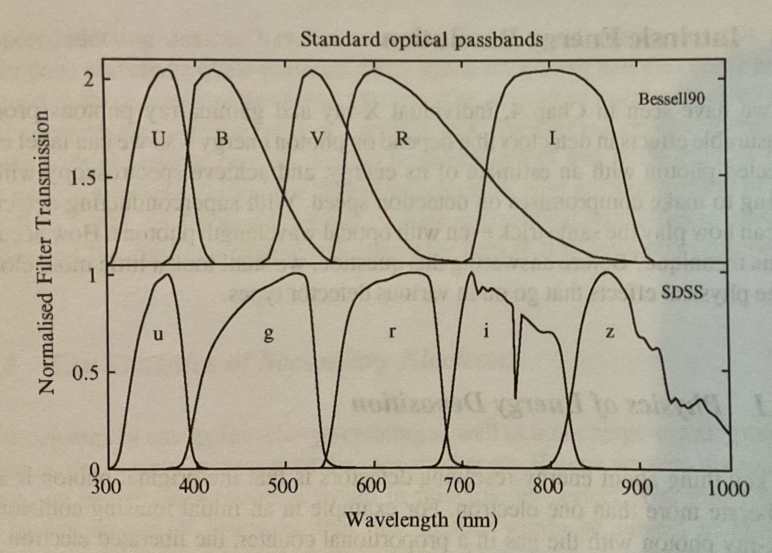
Fig. 9 Popular optical filtersets. The upper panel shows the UBVRI Johnson(-Cousins) passbands, while the lower panel shows the Sloan Digital Sky Survey (SDSS) \(ugriz\) passbands. Fig 5.3 from Lawrence’s Astronomical Measurements textbook.#
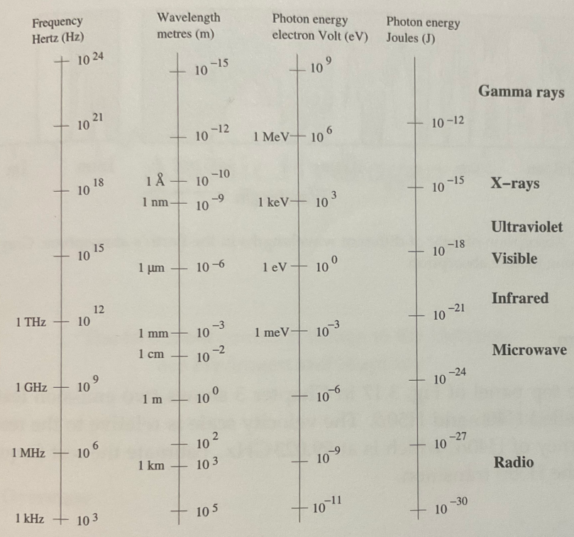
Fig. 10 Mapping between frequency, wavelength and energy across the electromagnetic diagram. Fig 2.4 from Tennyson’s Astronomical Spectroscopy textbook.#
For certain applications, high resolution spectroscopy is indispensable, such as Doppler shifts of parent stars host to exoplanets. The majority of spectroscopic observations on large ground-based telescopes are now devoted to medium resolution observations of highly-multiplexed instruments, involving either integral-field or multi-object spectroscopy For example, the upcoming 4MOST instrument at the VISTA telescope in Chile can observe 2400 sources simultaneously.
Units, notation and spectrographs#
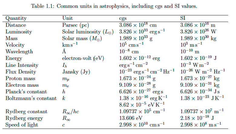
Astronomers generally favour cgs (cm, gram, sec) system over S.I. units as well as specialist units (pc for distances, brightness in mag). A summary of common units are presented in Table 1.1. Of these, the cgs unit of energy (erg) is likely to be the most unfamiliar (1 erg = 1 g cm2 s-2 = 10-7 J).
Measurements of spectra obtained in laboratories are usually reported in \(E/(hc)\) units (cm-1). These are directly proportional to the energy jump of the transition, \(E/(hc)\) = 8065 cm-1 (= 1 eV). In contrast, ultraviolet, optical and near-IR astronomers overwhelmingly favour wavelength units (Å equal to 10-10 m or μm equal to 10-6 m) and monochromatic fluxes in \(F_{\lambda}\) (erg s-1 cm-2 Å-1). Although our emphasis is on astronomical spectroscopy, we do refer to broad-band filters, so common filtersets (Johnson and Sloan) are shown in Fig. 9. Wavelengths are usually expressed in vacuum in the space ultraviolet, in air for the optical (the speed of light in a medium is less than in a vacuum, differences are small but non-zero). For example, the wavelength of the well known forbidden [O III] 4959Å line in a vacuum is 4960Å.
X-ray spectroscopists usually prefer kilo-electron Volt (keV) for energy versus photon rates per (kilo-)second (X-ray photons are rare), whereas radio observers favour ν (MHz or GHz) versus \(F_{\nu}\) (Jansky), recalling \(F_{\lambda} d\lambda = F_{\nu} d\nu\). A Jansky (abbreviation Jy) is named after radio pioneer Karl Jansky, and equals 10-23 erg s-1 Hz-1. Fig. 10 compares frequencies, wavelengths and energies across the electromagnetic spectrum.
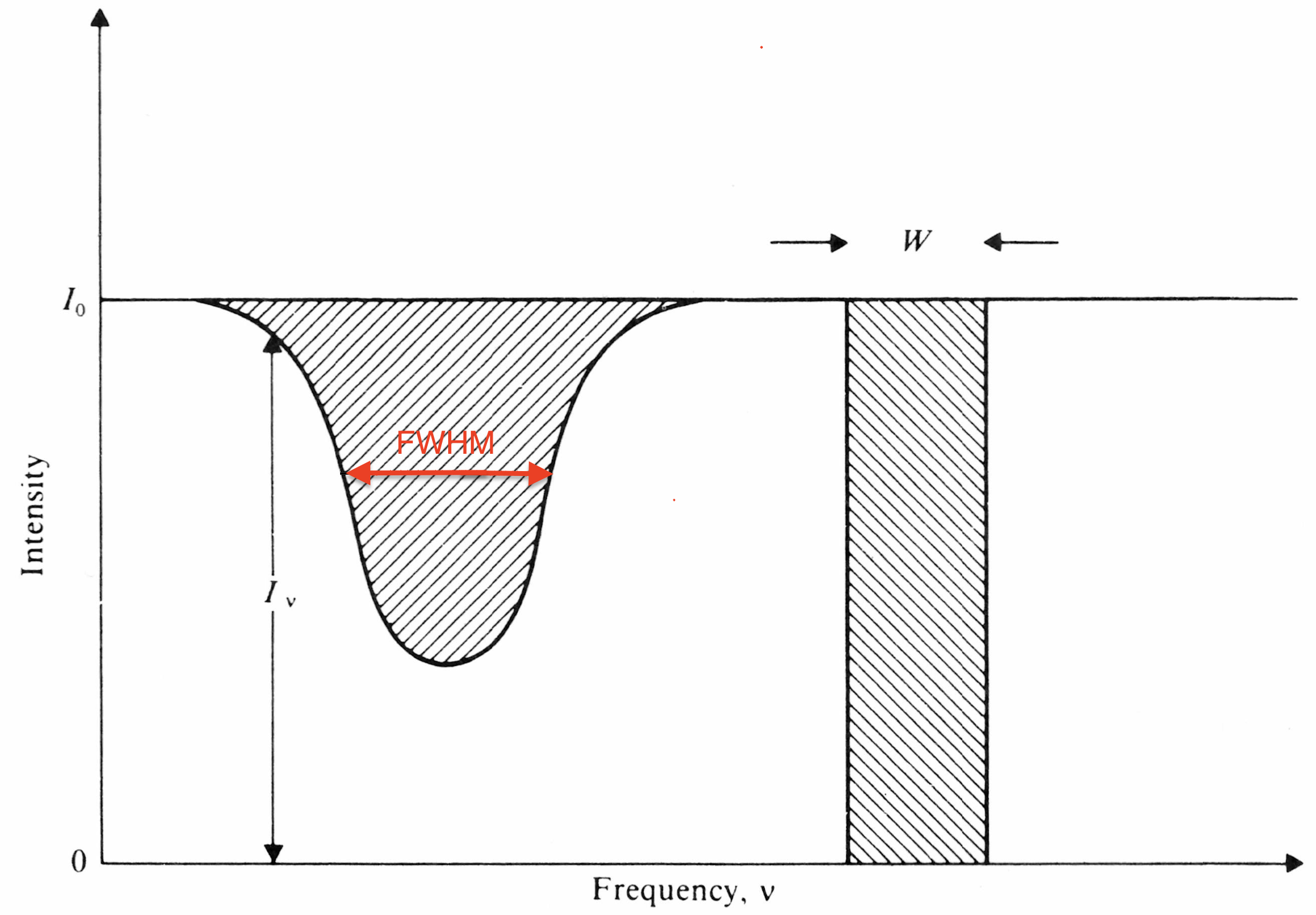
Fig. 11 The equivalent width, \(W_{\lambda}\), is defined so that the two shaded areas are equal (usually measured in Å at optical wavelengths), whereas FWHM (in red) is the line width at half intensity (usually measured in km s-1 at optical wavelengths). Figure adapted from Fig 2.2 of The Physics of the ISM (Dyson & Williams).#
Absorption lines, such as those shown in Fig. 8 are, somewhat confusingly, characterized in terms of their line strength as Equivalent Width (\(W_{\lambda}\)) and line broadening, via their Full-width at Half Maximum strength (FWHM). These are illustrated in Fig. 11. Equivalent widths are measured relative to a continuum so can be obtained for either absorption or emission lines in most circumstances, but cannot be defined for a pure emission line spectrum (e.g. Fig. 2), whereas line fluxes, \(F_{\lambda}\), can be measured in all instances if working with flux calibrated spectroscopy. Emission versus absorption lines are illustrated in Fig. 12. A detailed treatment of the latter will be deferred until PHY305 next year. It is the usual convention to list transitions as lower-upper state when discussing absorption lines in stellar atmospheres, but as upper-lower state when discussing emission lines.
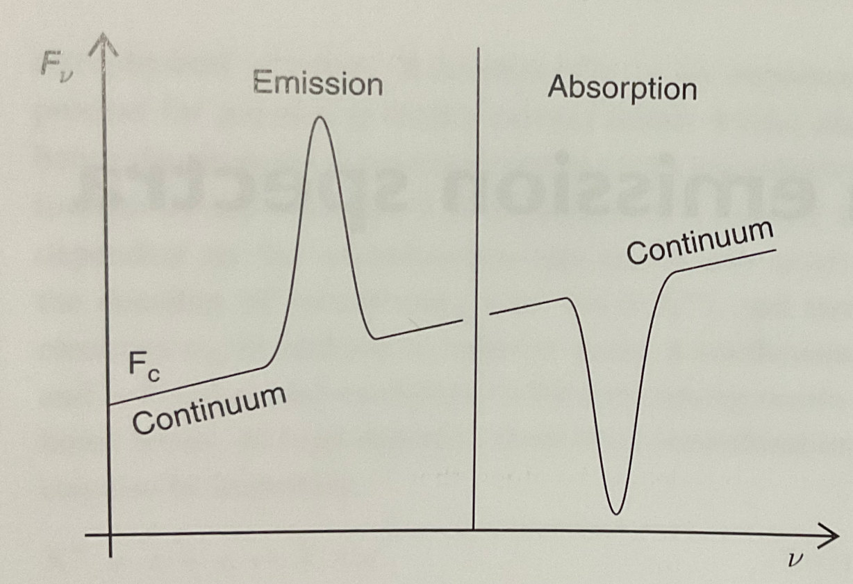
Fig. 12 Emission versus absorption lines relative to the continuum. Fig 8.1 from Pradhan & Nahar’s Atomic Astrophysics and Spectroscopy textbook.#
Figures 4-8 include identifications of specific spectral features. Lines from neutral species are denoted with the Roman numeral I (e.g. H I for neutral hydrogen), lines from singly ionized species are denoted II (e.g. He II, Fe II), so C CIV and Si IV correspond to lines of triply ionized carbon and silicon. The relevant ionization stages are H0, He+, Fe+, C3+ and Si+3+. Most features are known as ‘permitted’ transitions, but some are denoted with a trailing ] such as C III] at \(\lambda_0\) = 1909Å in Figs 4-6, which are known as ‘semi-forbidden’, while those with opening and closing square brackets such as [O III] at \(\lambda_0\) = 4363Å in Fig. 4 are known as ’forbidden’ lines. We will return to this topic in Chapter 3.
Example 1.1
Estimate the redshift and recession velocity of GN-z11
shown in Fig.4 from a comparison between the observed wavelength of
three emission lines and their rest-frame wavelengths.
Prominent emission lines include C III] λ1909, Mg iII2800Å
and Hδ at 4101Å
These lines are observed at \(\lambda_0\) = 2.2μm, 3.25μm and 4.75μm, resrespectivly so \(\Delta \lambda/\lambda_0\) = 10.5, 10.6 and 10.6. Adopting \(z\) = 10.57, \(v_{r}/c \sim 0.985\).
Example 1.2
What is the theoretical angular resolution of the pt5m telescope (diameter 0.5m) on La Palma in the V-band in arcsec. Why is this not achieved in practice?
V-band corresponds to 0.55μm, so θ = 0.275 arcsec. In practice, atmospheric turbulence affects image quality, even at good observing sites like La Palma.