Chapter 4: Interstellar medium

We have discussed the effects of atmospheric extinction in Chapter 2. In addition, the interstellar (intergalactic beyond the Milky Way) medium (ISM) affects fluxes received at the top of our atmosphere. For UV and optical light, dust (1% of the ISM by mass) plays the most significant role, whereas interstellar gas (99% of the ISM by mass) attenuates extreme UV and X-ray light. The density of material within the ISM is lower than the most perfect vacuum ever created in laboratories on Earth, so it is common to quote values in terms of the atom number density since the average over the entire Milky Way is \(\sim 1\) cm^-3. Characteristics of the gaseous phases of the ISM are summarised in Table 5. Further reading:

• Physics of the Interstellar and Intergalactic Medium, Bruce Draine, Princeton Series in Astrophysics

• Astrophysics of Gaseous Nebulae and Active Galactic Nuclei, Donald Osterbrock, & Gary. Ferland, University Science Books

• Atoms, stars and nebulae, Lawrence Aller, Cambridge

Table 5 Characteristics of the gaseous phases of the ISM in the Milky Way, from Table 1.1 of A. Tielens’ Physics and Chemistry of the ISM.

Phase	\(n\) (cm -3)	\(T\) (K)	\(M (10^{9} M_{\odot}\))	Location
Hot	0.003		–	Halo
Warm ionized	0.1	8000	1.0	Thick disk
(HII)	\((1-10^{5})\)	\((10^{4})\)	(0.05)	(Thin disk)
Warm neutral	0.5	8000	2.8	Thick disk
Cold neutral	50	80	2.2	Thin disk
Molecular	\(> 200\)	10	1.3	Thin disk

The Galactic distribution of H  i (from 21cm) was shown in Fig. 64, revealing it to be highly concentrated in the Galactic disk. A similar representation of dust (from COBE and IRAS) is shown in Fig. 84 revealing a similar distribution.

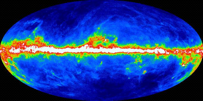
Fig. 84 100μm dust map of the sky from Schlegel et al. (1998) in Aitoff projection (Galactic centre in middle), reminiscent of the distribution of hydrogen gas from Fig. 64

Table 6 A comparison of UV, optical and IR extinctions ,\(x_{\lambda} = A_{\lambda}/A_{V}\) for a standard \(R_{V} =3.1\) extinction law from Seaton (1979, S79) and Cardelli et al. (1989, CCM89).

Filter	\(\lambda (\mu\)m)	\(A_{\lambda}/A_{V}\) (S79)	\(A_{\lambda}/A_{V}\) (CCM89)
	0.150	2.796	2.664
	0.218	3.174	3.180
	0.333	1.601	1.644
[O  II]	0.373	1.471	1.539
Hγ	0.434	1.320	1.347
[O III]	0.436	1.313	1.338
Hβ	0.486	1.171	1.164
[O III]	0.501	1.129	1.120
V	0.555	0.984	0.989
Hα	0.656	0.796	0.818
[N  II]	0.658	0.793	0.815
[S  II]	0.672	0.770	0.793
	1.00	0.413	0.404
Pα	1.87	0.131	0.147
	2.20	0.095	0.114

Dust absorption

Dust comprises sub-micron sized particles (silicate or carbonaceous) which absorb or scatter light, especially at ultraviolet and optical wavelengths. The volume density of dust is low, so nearby stars at parsec distances are relatively unaffected, but distant sources are severely impacted, especially towards the Galactic Centre, and appear redder than they would without interstellar dust, since dust preferentially absorbs/scatters shorter wavelengths.

Considering broad-band \(B\) (\(\sim\)4400Å) and \(V\) (\(\sim\)5500Å) photometric filters if the intrinsic colour of a star is \((B-V)_0\) and the observed colour is \(B-V\), then the difference, the colour excess \(E_{B-V} = (B-V) - (B-V)_0 = A_B - A_V\) . The amount of visual dust extinction \(A_{V}\) (in mag) is

\[A_{V} = R_{V} \times E_{B-V}\]

where \(R_{V} \sim 3.1\) for a standard Milky Way extinction law.

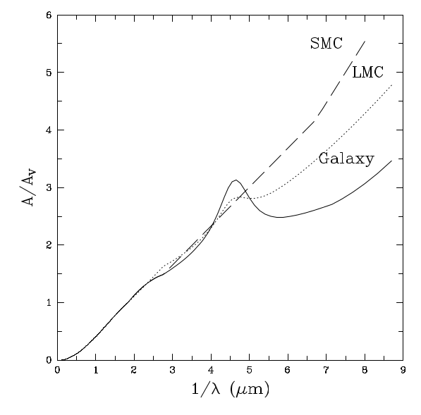
Fig. 85 Average wavelength dependence of extinction law (\(A_{\lambda}/A_{V}\)) versus reciprocal wavelength (\(1/\lambda\)) for Milky Way (solid), LMC (dotted) and SMC (dashed) sight-lines, following Seaton (1979), Howarth (1983) and Bouchet et al. (1985). The broad feature at 4.6 μm^-1 is thought to be due to carbon-based dust.

UV to IR extinction law

Robert Trumpler (1930) first recognised that there is a material between the stars from analysis of the angular size of open clusters. The amount of light from a source shining through interstellar dust is reduced according to

(26)\[F_{\lambda} = I_{\lambda} \exp (-\tau_{\lambda})\]

where \(F_{\lambda}\) is the observed flux, \(I_{\lambda}\) is the intrinsic flux and \(\tau_{\lambda}\) is the optical depth. Dust extinction can also be measured in magnitudes via

(27)\[\frac{A_{\lambda}}{\rm mag} = 2.5 \log (I_{\lambda}/F_{\lambda})\]

so the extinction in magnitudes \(A_{\lambda}\) is proportional to optical depth \(\tau_{\lambda}\),

(28)\[A_{\lambda} = 2.5 \log (\exp \tau_{\lambda}) = 1.086 \tau_{\lambda}.\]

The latter can be expressed in terms of the properties of dust grains and path length as follows

(29)\[\tau _{\lambda} = n_d \pi a^{2} Q_{\rm ext} L\]

where \(n_d\) is the number density (cm^-3) of dust grains, each of size \(a\) (typically within an order of magnitude of 0.1 μm), \(Q_{\rm ext}\) is the efficiency factor of extinction (sum of absorption and scattering efficiency factors) and \(L\) is the path length. Detailed discussion of grain properties is provided in Draine’s Physics of the Interstellar and Intergalactic Medium textbook.

Since we are focused on spectroscopy, we would like to know the wavelength dependence of extinction, \(A_{\lambda}\), especially in the UV and optical. This has been determined from the spectral energy distributions of pairs of unreddened and reddened stars of the same spectral type. Extinction can be expressed as a reddening law

\[\tau_{\lambda} = C x_{\lambda}\]

where the factor \(C\) depends on the star, but \(x_{\lambda}\) is approximately the same for most stars in the Galaxy. These equations can be combined as

\[F_{\lambda} = I_{\lambda} 10^{-\log e C x_{\lambda}} = I_{\lambda} 10^{-0.434 C x_{\lambda}} = I_{\lambda} 10^{-c x_{\lambda}}\]

where \(c = 0.434 C\). From the definition of magnitude Eqn (27), \(A_{\lambda} = 2.5 c x_{\lambda}\). \(x_{\lambda} = A_{\lambda}/A_{V}\)

is shown in Fig 85 follows Seaton (1979) although Cardelli, Clayton & Mathis (1989, CCM) is also widely used in the literature.

Table 6 compares UV, optical and IR \(x_{\lambda}\) coefficients for a standard Seaton or CCM \(R_{V} = 3.1\) law. \(A_{\lambda}/A_{V} \sim 2\) in the near-UV (with a prominent feature at \(1/\lambda = 4.6 \mu\)m^-1) and \(A_{\lambda}/A_{V} \sim 3\) in the far-UV. Near-IR extinction is significantly lower than at UV or optical wavelengths (e.g. \(A_{K}/A_{V} \sim 0.1\)) and follows an approximate power law \(A_{\lambda} \propto \lambda^{-1.6}\) according to Rieke & Lebofsky (1985), although there are discrete features in the IR extinction law analogous to the UV feature (notably 9.7μm due to silicate dust).

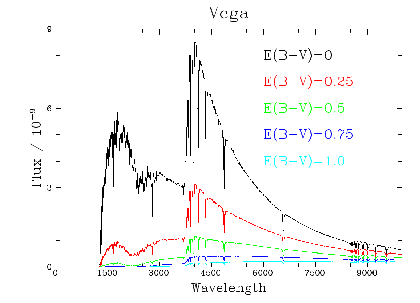
Fig. 86 UV and optical flux distribution of Vega (A0 V) based on Kurucz ATLAS model, together with varying amounts of dust extinction \(E_{B-V}\)=0.25 (red), 0.50 (green), 0.75 (blue), 1.000 (cyan).

Figure 86 presents the UV to optical flux distribution of Vega, based on Kurucz ATLAS models, together with the effect of increasing dust extinctions, E_B-V=0.25, 0.50, 0.75 and 1.00 for a standard Galactic extinction law. The broad UV feature in the law at Fig. 85 leads to a lower resulting flux at λ=2200Å. Differences in dust properties in the metal-poor Large and Small Magellanic Clouds are also illustrated, revealing higher UV dust extinction for the same amount of visual extinction.

In this course we largely focus on line emission, so dust extinctions across broad-band filters are not particularly useful. Instead, for nebular studies in the visual, Hβ is used as a reference, i.e..

(30)\[\frac{F_{H\beta}}{I_{H\beta}} = 10^{-c_{H\beta} x_{H\beta}}\]

so

(31)\[\frac{F_{\lambda}}{F_{H\beta}} = \frac{I_{\lambda}}{I_{H\beta}} 10^{-c_{H\beta} (x_{\lambda} - x_{H\beta})}.\]

If pairs of intrinsic line ratios are known, it is possible to measure extinction via \(c_{H\beta}\) since tabulated values of \(x_{\lambda} = A_{\lambda}/A_{V}\) are known (e.g. Table 6). We will exploit this relation when determining extinction towards H II regions in the next Chapter.

Gas absorption

Hydrogen gas impacts on spectroscopy via interstellar Lyman absorption lines and (severe) attenuation of extreme UV and soft X-ray fluxes. Other elements also imprint on the UV and optical spectrum, as well as molecular hydrogen.

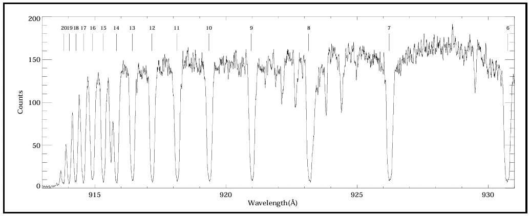
Fig. 87 Lyman interstellar lines (labelled) superimposed on the FUSE spectrum of a nearby hydrogen-rich White Dwarf WD2211-495, from Sahnow et al (2000).

Interstellar lines in the UV and optical

Johannes Hartmann (1904) first recognised that absorption lines were present in the ISM from spectroscopic observations of the binary δ Ori. Doppler shifts of Balmer lines from the brighter component followed the orbit, but Ca II H and K lines remained stationary. These together with Na I D lines, first identified in the ISM by Mary Lea Heger in 1919, are the strongest optical ISM absorption lines superimposed on stellar spectra. We have previously introduced the equivalent width, \(W\), of a line (Fig. 11). Mathematically this can be expressed as

\[W_{\nu} = \int \left(1 - \frac{I_{\nu}}{I_{\nu,0}} \right) d\nu.\]

where \(I_{\nu,0}\) and \(I_{\nu}\) are the intensity of radiation before and after absorption. We will defer a full discussion of the radiative transfer equation until next year (PHY305) but the parallel-ray case (for negligible emission processes) is

(32)\[\frac{d I_{\nu}}{ds} = - \kappa_{\nu} I_{\nu}\]

where \(\kappa_{\nu}\) is the (wavelength dependent) absorption coefficient per unit path length (\(s\)). If we define optical depth, \(\tau_{\nu}\) as

\[\tau_{\nu} = \int \kappa_{\nu} ds\]

then the integral of Eqn (32) is \(I_{\nu} = I_{\nu,0} \exp (-\tau_{\nu})\), so in the optically thin (small \(\tau_{\nu}\)) limit where \(\exp (-\tau_{\nu}) \sim 1 - \tau_{\nu}\) so

\[W_{\nu} = \int 1 - (1 - \tau_{\nu}) d\nu = \int \tau_{\nu} d\nu.\]

If we now introduce a cross section, \(\sigma_{\nu}\) the total absorption becomes \(\tau_{\nu} = N \sigma_{\nu}\) where \(N\) is the total number of absorbers, so

\[W_{\nu} = N \int \sigma_{\nu} d{\nu} = N \sigma_{0} \Delta \nu\]

where \(\sigma_0\) is the mean cross-section over the bandwidth \(\Delta \nu\). For optically thin lines, if \(\sigma_0\) is known we may derive the column density \(N\) (in cm^-2) of atoms causing the line. Lines become saturated at high column densities, so a so-called curve of growth approach is needed to determine \(N\).

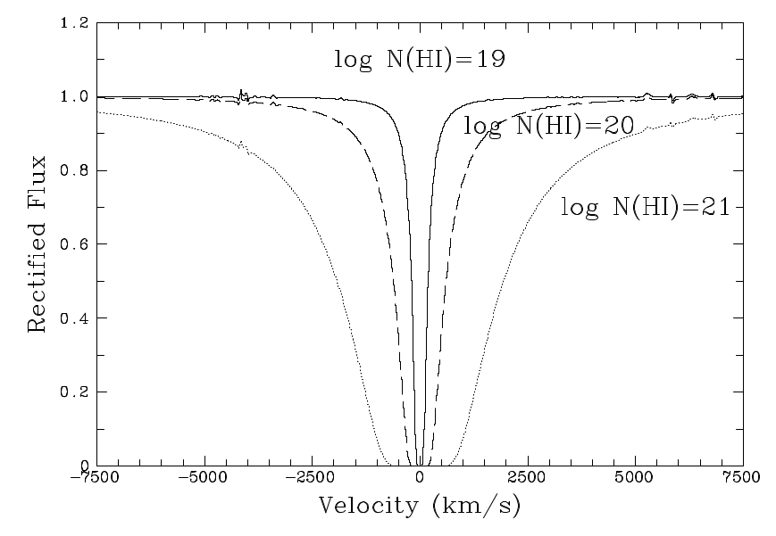
Fig. 88 Theoretical Lyman α profiles for a range of \(N(H)\) column densities (in cm^-2).

In the space ultraviolet, there are numerous interstellar absorption lines, notably the Lyman series, allowing a direct measurement of the atomic hydrogen column density against background hot stars (needed to show a strong continuum in the far-UV). Fig. 87 shows high members of the interstellar Lyman series against FUSE spectroscopy of a DA-type white dwarf. Theoretical Ly α profiles for a range of atomic hydrogen column densities, \(N_{H}\) are presented in Fig. 88. Armed with hydrogen column densities from Lyman α fits, and \(A_{V}\) from spectral energy distributions, it is possible to determine typical values of the extinction per unit H column density of \(A_{V}/N_{H} \sim 5.3 \times 10^{-22}\) mag cm² H^-1. The connection between \(A_{V}\) and total number of H atoms along the line of sight can be expressed via Eqn (29) as

\[% Kwok A_{V} = 1.086 \frac{n_d}{n_{H}} \pi a^{2} Q_{\rm V} N_{H}\]

where \(Q_{\rm V}\) is the extinction efficiency at the V-band, so empirical results allow the dust-to-gas number ratio \(n_{d}/n_{H}\) ito be obtained.

Similar relations hold for sight-lines towards the Magellanic Clouds, except that the reddening per H atom is reduced (Koornneef 1982, Fitzpatrick 1985).

In addition, series of H₂ molecular lines can also be seen between Ly α and the Ly edge (912Å). These are, somewhat confusingly, known as Lyman-Werner bands, and allow \(H_{2}\) column densities to be determined from far-UV spectroscopy (e.g. FUSE satellite). Molecules have a far more complex structure than atoms since there is no single charge centre about which electrons move, and the nuclei themselves move, giving rise to both rotational and vibrational motions. You will be relieved that we will not discuss molecules in this course, although Tennyson’s Astronomical Spectroscopy textbook is a good place to find out more. Metal interstellar lines spanning neutral (e.g. N I), single ionized (e.g. C II, Mg II) and highly ionized high (e.g N V, O VI) ions are observed in the far UV, indicating that the interstellar medium spans a wide range of temperatures.

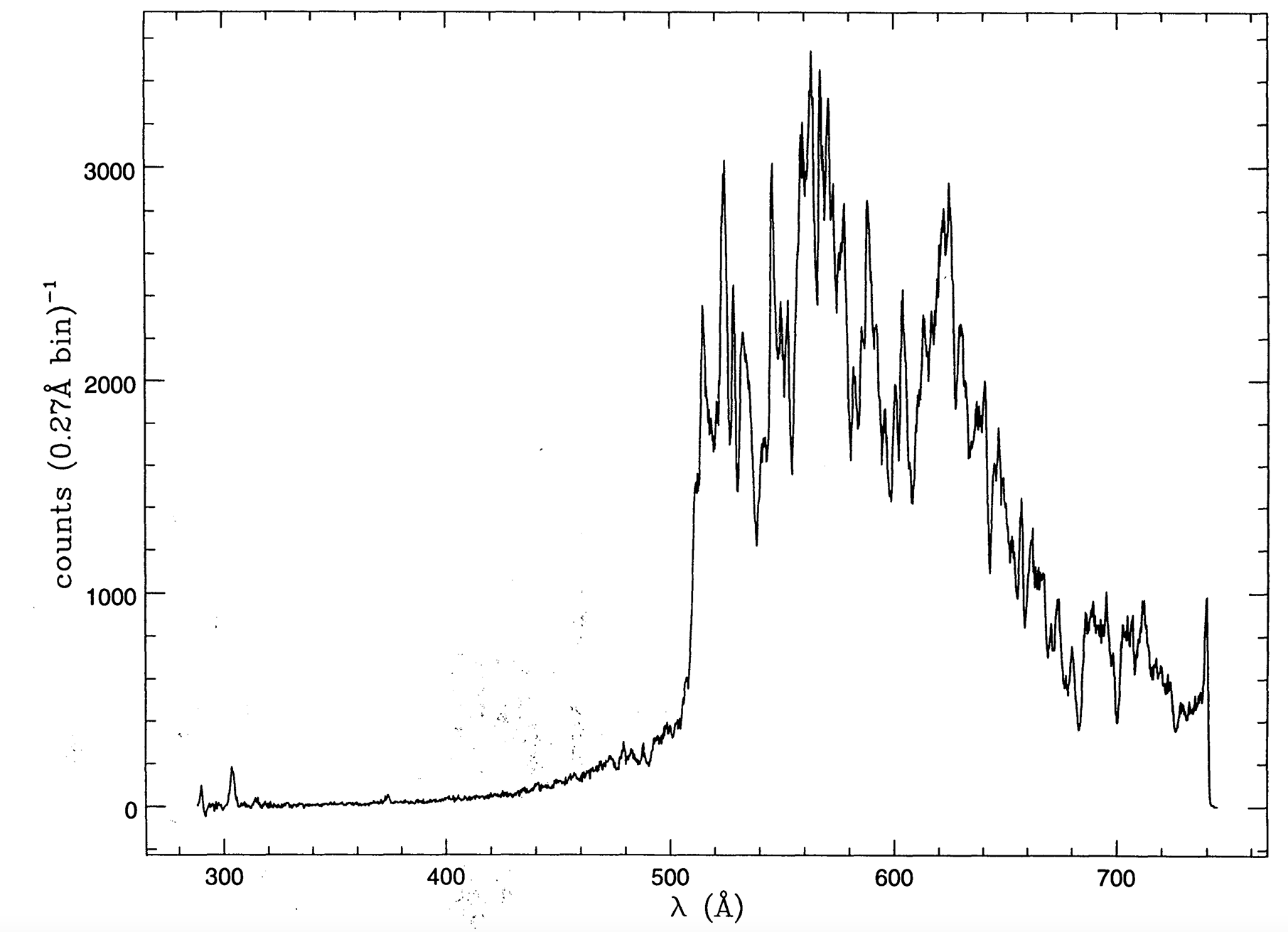
Fig. 89 Extreme UV observations of the B star ε CMa with EUVE owing to a very low hydrogen column density towards this star. Cassinelli et al. (1995). The emission line at 303Å is He II Ly α.

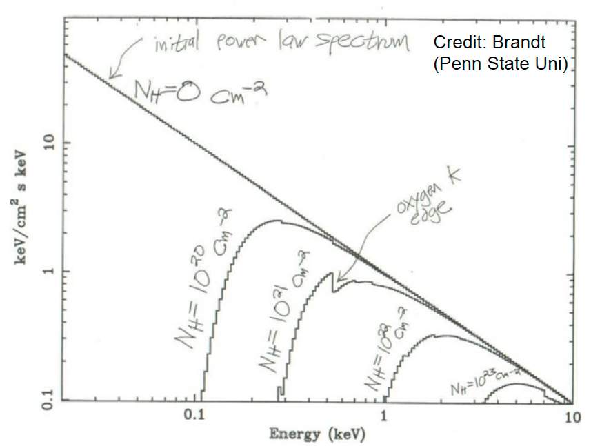
Fig. 90 Absorption of an initial power law X-ray spectrum due to increasing hydrogen column densities (in cm^-2). Credit: Brandt (Penn State).

Hydrogen absorption in the Lyman continuum

Interstellar dust absorbs/scatters UV and optical light, whereas interstellar hydrogen gas absorbs energetic photons in the extreme UV (EUV) and soft X-rays. Hot stars emit large amounts of photons with energies above 13.6 eV (\(\lambda <\) 912Å) but if there is a significant column density of hydrogen atoms between the source and the top of the Earth’s atmosphere, the entire EUV flux is absorbed. Since dust and gas are well mixed, there is relatively little dust or gas on scales of tens of parsec, but for most sight-lines at scales of ≥100 pc EUV observations are not possible. Exceptions exist, such as the low column density of \(N(H) = 10^{18}\) cm^-2 towards the hot star ε CMa (\(d\) = 200 pc) for which EUVE spectroscopy is shown in Fig. 89.

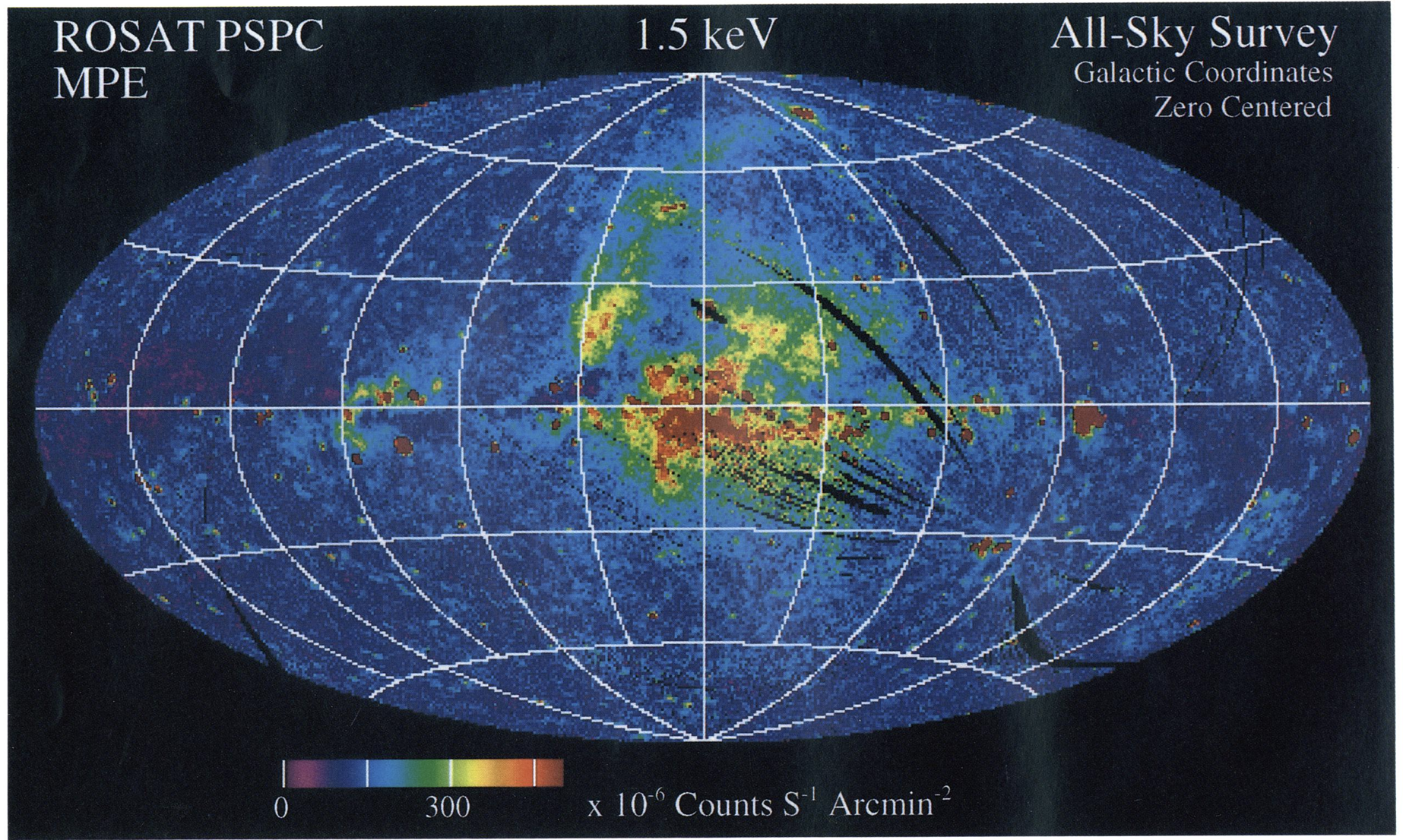
Fig. 91 ROSAT 1.5 keV X-ray map of the sky from Snowden et al. (1995) in Aitoff projection (Galactic centre in middle), showing X-ray emission extending into the Galactic halo.

Gas attenuation extends into the soft X-ray regime. Active Galactic Nuclei are sources of prodigious emitters of X-rays with a power law slope. This is illustrated in Fig. 90 which shows the effect of different hydrogen column densities. Hard X-ray photons (several keV) are barely attenuated at high column densities, whereas soft X-ray photons (\(\ll 1\) keV) are severely attenuated at modest column densities of \(N(H) \sim 10^{21}\) cm^-2 (\(A_{V} \sim\) 0.5 mag).

We have previously shown the Galactic distribution of H i (Fig. 64) and dust (Fig. 84), both of which are highly concentrated in the Galactic disk (the same is true of molecular gas). In contrast, hot (coronal) gas extends into the Galactic halo, as illustrated in Fig. 91 which shows the ROSAT all-sky 1.5 keV view.

Example 4.1

Question

Suppose that the ISM contains dust grains with uniform number density \(10^{-12}\) cm^-3, all with the same radius, \(10^{-1} \mu\)m, and extinction efficiency \(Q_{\rm ext}\) = 0.5 at wavelength \(\lambda_{0}\). Find the extinction in magnitudes at wavelength \(\lambda_0\) for a star at a distance 1 kpc from Earth.

Solution

From Equation (28), \(A_{\lambda} = 1.086 \tau_{\lambda}\) and inserting values into Eqn (29) \(A_{\lambda} = (1.086) (10^{-12}) \pi (10^{-5})^{2} (0.5) (3.086 \times 10^{21}) = 0.53\) mag.

Example 4.2

Question

A distant HII region in the Milky Way is found to have a Balmer recombination line flux ratio \(F_{H\alpha}/F_{H\beta}\) = 4.0. Given that Case B recombination theory predicts a ratio of 2.86 for this pair of lines at typical \(n_{e}, T_{e}\), calculate the de-reddening factors by which the observed line fluxes must be multiplied to remove the effects of extinction.

Solution

From Eqn (37), \(c_{H\beta} = 0.42\) (CCM law), so from Eqn (30), \(I_{H\beta}/F_{H\beta} = 10^{c_{H\beta} x_{H\beta}} = 10^{0.42 \times 1.164} = 3.09\), and \(I_{H\alpha}/F_{H\alpha} = 10^{c_{H\beta} x_{H\alpha}} = 10^{0.42 \times 0.818} = 2.21\). By way of sanity check, \(4.0 \times 2.21/3.09 = 2.86\) as expected.

Example 4.3

Question

Compare the lifetime of the hydrogen 21cm hyperfine transition to the age of the Universe. why do we see the line at all?

Solution

The Einstein A value for 21cm is \(2.9 \times 10^{-15}\) s^-1 from Table 3.1 so its mean lifetime is \(1/A = 3.4\times 10^{14}\) s or 11 Myr. This is \(\sim\)0.1% of the age of the Universe (13.8 Gyr), but is observed so readily since there are so many hydrogen atoms in the Milky Way (and other galaxies).