
Chapter 3: Atomic Physics#
Atomic (and molecular) physics and astrophysics have developed together over centuries since our understanding of planets, stars, nebulae and galaxies relies on detailed spectroscopic analysis of the atoms they contain. You will come across a full quantum mechanical treatment of atomic structure elsewhere (PHY21005, PHY332). Further reading:
Astronomical Spectroscopy, J. Tennyson, World Scientific
Astrophysics of Gaseous Nebulae and Active Galactic Nuclei, D. Osterbrock & G Ferland, University Science Books
Here we use the Bohr model for hydrogen-like ions, plus selection rules with application specifically to nebulae, which will be discussed in depth in Chapter 5.
An atom in an excited state has a spontaneous tendency to de-excite by a radiative transition involving the emission of a photon (atoms with excess energy tend to want to get rid of it). This process is called spontaneous emission. Consider a transition from an upper level \(u\) to a lower level \(l\). Let us suppose there are \(N_u\) atoms in the upper level at time \(t\). The rate equation for \(N_u\) is
i.e. the number of atoms making transitions is proportional to the number of atoms in the excited state and the quantum mechanical probability. The parameter \(A_{ul}\) is determined by the transition probability and gives the spontaneous decay rate. It is called the Einstein A coefficient.
The solution to Eqn (10) is
where \(\tau = 1/A_{ul}\).This shows that the population of atoms in the upper level will decay by spontaneous emission with a time constant τ, the radiative lifetime of the excited state. The values of \(A_{ul}\), and hence τ vary considerably from transition to transition.
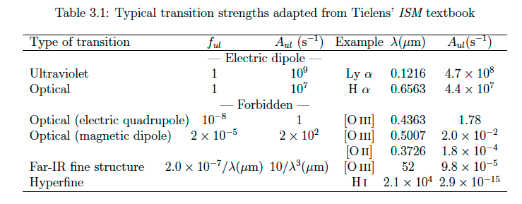
Fig. 58 Typical transition strengths adapted from Tielens’ ISM textbook#
Examples of Einstein \(A\) coefficients for permitted and forbidden lines common in astrophysics are shown in Figure 58 a.k.a. Table 3.1. Allowed transitions (‘E1’) have Einstein \(A\) coefficients in the range to s-1, giving radiative lifetimes in the 1 μs to 1 ns range. Forbidden transitions are much slower with Einstein \(A\) coefficients in the range to s-1 range, so radiative lifetimes are in the milli-second range or longer (0.6 sec for [O III] 4363Å). Fine structure lines possess very long radiative lifetimes (several hours for [O III] 52μm), while hyperfine transitions possess exceptional radiative lifetimes (11.5 million years for the 21 cm line).
Hydrogen atom#
Let us recall the semi-classical Bohr model for line emission from atoms, in which electrons could only occupy certain orbital radii, \(r_n\) (satisfying angular momentum, \(L = nh/(2\pi)\) (where \(n = 1, 2, 3, \ldots\))
where the Bohr radius \(a_0 (5.29 \times 10^{-11}\) m) is
The total energy of the \(n^{th}\) orbit is the sum of kinetic and potential terms:
where \(R^{\prime}\) is given by
in which μ is the reduced mass and the Rydberg energy (13.606 eV) is
\(R_{\infty}/(hc)\) is the Rydberg constant (109,737 cm-1), named after Johannes Rydberg (1854-1919). Therefore, the integer \(n\), known as the principal quantum number completely determines the radius and energy of each orbit of the Bohr atom. When the electron is in the lowest energy level (\(n=1\) - the ground state), its energy is simply \(E=-R^{\prime}\). Since it would take an amount of energy equal to \(R^{\prime}\) to remove the electron from the atom; \(R^{\prime}\) is the ionisation energy of the atom, and scales with the square of the atomic number.
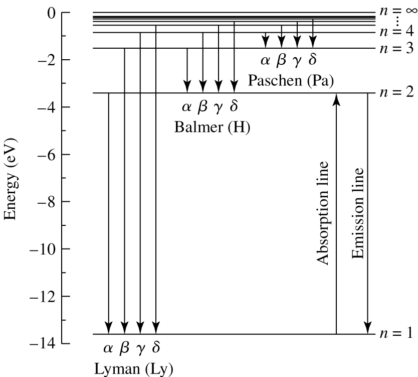
Fig. 59 Energy level diagram for a hydrogen atom showing the Lyman, Balmer and Paschen lines (downward arrows indicate emission lines; upward arrows indicate absorption lines).#
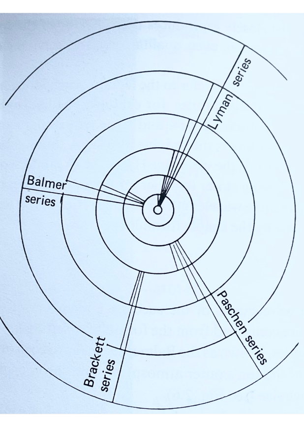
Fig. 60 Bohr model of the Hydrogen atom, showing Lyman, Balmer, Paschen and Brackett series. From Aller’s Atoms, Stars and Nebulae textbook.#
\(R^{\prime}\) is the effective energy of the system in question. For hydrogen we have an electron, of mass \(m_{e}\) orbiting a proton of mass m\(_{p} (\sim 1836 m_{e}\)) so the reduced mass μ is given by
so the effective Rydberg energy for hydrogen is
When an electron moves between one orbit and another, it emits or absorbs a photon. The energy of the photon is given by the difference in energy between the two orbits, \(\Delta E = E_{n_1}-E_{n_2}\). Equation (14) leads to an equation for the energy of the emitted or absorbed photon
Since, for a photon \(E=h\nu\), the corresponding frequency of the photon is
And, finally, we can use the wave equation \(\nu \lambda = c\) to obtain the wavelength of the photon as
where \(R_{H}/hc\)= 109,677 cm-1. This equation give the wavelength of the radiation that would be emitted/absorbed when electron jumps from one level to another.
When an electron jumps from the \(n=2\) orbit to \(n=1\) level, a photon of wavelength \(\lambda = \frac{ch}{R_{\rm H}} \left( \frac{1}{1} - \frac{1}{4} \right)^{-1} = 1216\)Å is emitted. The reverse process can also occur; an electron in the \(n=2\) orbit can absorb a photon of wavelength 1216Å and jump to the \(n=2\) orbit.
Considering the energy levels in more detail, it is clear that the line spectrum of hydrogen will exhibit a number of “series”, associated with transitions to and from a given orbit. For example, transitions from the \(n=2,3,4,\ldots,\infty\) energy level to the \(n=1\) level cause a series of emission lines known as the Lyman series. The line we considered above, when the electron jumps from \(n=2\) to \(n=1\) is part of the Lyman series. In fact, it is the first line of the Lyman series, Ly α, in the far ultraviolet part of the spectrum. This series is illustrated in an energy level diagram Fig. 59.
There are also series of lines in the optical, corresponding to transitions to and from the \(n=2\) state (the Balmer series, usually indicated with a H for hydrogen, as in Fig. 1), followed by transitions to and from the \(n=3\) orbit (the Paschen series), the \(n\)=4 orbit (the Brackett series) and so on, as illustrated in Fig. 60 and summarised in Table 1, which includes their discoverers. Higher series are unnamed (Peter Hansen & John Strong demonstrated the seventh series experimentally in 1972).
\(n_{\rm low}\) |
Discoverer |
Symbol |
Spectral region |
α |
limit |
1 |
(Theodore) Lyman |
Ly |
Far-ultraviolet |
1215Å |
912Å |
2 |
(Johann) Balmer |
H |
Optical |
6563Å |
3646Å |
3 |
(Friedrich) Paschen |
P |
Near IR |
1.87 μ m |
8205Å |
4 |
(Frederick) Brackett |
Br |
Near IR |
4.05 μ m |
1.46 μ m |
5 |
(August) Pfund |
Pf |
Near-mid IR |
7.46 μ m |
2.28 μ m |
6 |
(Curtis) Humphreys |
Hu |
mid-IR |
12.4 μ m |
3.28 μ m |
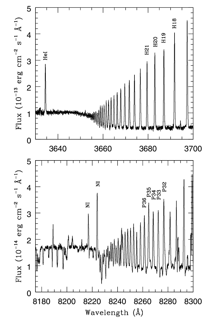
Fig. 61 Nebular emission lines of hydrogen in the Orion nebula in the vicinity of the Balmer (upper) and Paschen (lower) limits. From Esteban et al (2004).#
Look at the spacing of the energy levels in Fig 59, and compare it to Eqn (14). As \(n\) increases, the energies of the orbits become more closely spaced. Therefore the difference in energy, or frequency, or wavelength between successive lines in a series gets smaller as \(n\) increases. Eventually, the spacing of the energy levels approaches zero, and the emission or absorption lines get very closely spaced indeed. We say the series has reached its limit. Balmer and Paschen series limits are shown in Fig. 61 for the Orion Nebula.
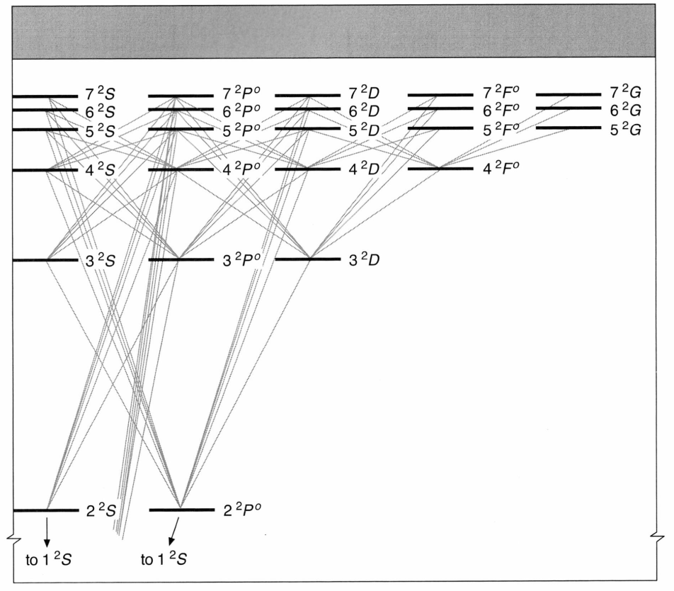
Fig. 62 Partial energy-level diagram for neutral hydrogen, limited to \(n \leq 7\) and \(l \leq 4\). Permitted radiative transitions to levels \(n < 4\) are indicated by solid lines. Figure 2.1 from Osterbrook & Ferland’s AGN2 textbook.#
In reality, the structure of hydrogen is a little more complicated than presented so far. It is traditional to order interactions that occur inside atoms into a three-level hierarchy according to (i) gross structure (kinetic energy of electrons, Coulomb force), (ii) fine structure (spin-orbit interactions); (iii) hyperfine structure (nuclear interactions). The relevant quantum numbers of individual electrons within atoms are
Principal quantum number, \(n (= 1, 2, 3, \ldots\))
Orbital angular momentum, \(l = 0, 1, 2, \ldots, (n-1)\)
Magnetic quantum number, \(m_{l} = 0, \pm 1, \pm 2, \ldots, \pm l\)
where \(m_{l}\) is the component of the orbital angular momentum in one fixed direction. In general the gross energy of the electron is determined by \(n\) and \(l\). The degeneracy of each \(l\) state is \(2(2l+1)\), due to the Pauli exclusion principle, so for a given quantum number \(n\) the degeneracy is \(2 \sum_{l=0}^{n-1} (2l+1) = 2 n^{2}\).
Labels given to orbital angular momentum (which predated quantum mechanics) are
\(l=0 \rightarrow s\) (‘sharp’)
\(l=1 \rightarrow p\) (‘principal’)
\(l=2 \rightarrow d\) (‘diffuse’)
\(l=3 \rightarrow f\) (“fundamental’)
\(l=4, 5, 6 \ldots \rightarrow g, h, i\) (alphabetical)
Uniquely for hydrogen and hydrogen-like ions, \(E\) depends only on \(n\) (Eqn (14)). Fig 62 shows this more realistic energy level diagram for hydrogen, in the form of a Grotrian diagram (named after Walter Grotrian, 1890-1954), with \(l = 0, 1, 2, 3, 4\) levels separated in the \(x\)-axis, and the \(y\)-axis still displaying energy (increasing vertically). The parity is also straightforward for single electron systems, since it is ‘even’ or ‘odd’ depending on whether \(l\) is even or odd.
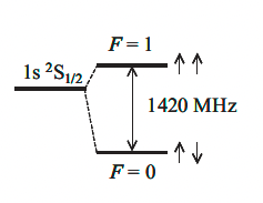
Fig. 63 Hyperfine structure of the \(1s\) ground state of hydrogen. The arrows indicate the relative directions of the electron and nuclear spin. Adapted from Figure 7.7 of Mark Fox’s Atomic Physics textbook.#
The ground state of atomic hydrogen, \(n\) = 1 implies \(l = 0\) so its configuration is \(1s\). Levels associated with \(n = 2\) have \(l = 0,1\) (configurations \(2s, 2p\)). For hydrogen and hydrogen-line ions, permitted transitions involve \(\Delta l = \pm 1\), so the grey lines in Fig. 62 connect permitted transitions of atomic hydrogen. Permitted transitions have large electric-dipole transition probabilities (Einstein \(A\) coefficients). Consequently, transitions between the \(1s\) and \(2p\) are permitted (\(\Delta l = 1\)) whereas transitions between \(1s\) and \(2s\) are not permitted (\(\Delta l = 0\)).
We also need to consider the spin angular momentum \(s\) of the electron. For a single electron \(s = 1/2\) so the component of the spin angular momentum \(m_{s} = -1/2\) (spin down) or \(m_{s} = 1/2\) (spin up) The addition of orbital and spin angular momenta is relatively straightforward, since the total angular momentum \(j\) is the vector sum of \(l\) and \(s\) – so can take integer values between \(| l-s | \leq j \leq | l+s|\) – fine structure levels involve a common term (\(n, l\)) but different \(j\) values. Selection rules for fine-structure transitions are \(\Delta j = 0, \pm 1\). The \(1s\) ground state of hydrogen has \(j = 1/2\) whereas the \(2p\) state has two sub-levels (\(j = 1/2\) and 3/2. Consequently there are two fine structure transitions within Lyα. However, the velocity shift between these transitions is so small (1.3 km s-1) that they are always blended due to thermal broadening, so in practice they are treated as a single \(1s-2p\) transition.
In most cases we need only concern ourselves with the fine structure of atoms, but occasionally, hyperfine structure needs to be considered too, which arise from interactions between the magnetic dipole due to the nuclear spin and the magnetic field produced at the nucleus by the electrons. The nuclear spin quantum number \(I\) can take integer or half-integer values, so the total angular momentum \(F\) of the whole atom (nucleus plus electrons) is \(F = I + J\) (\(J\) is the total electron angular momentum, identical to \(j\) for a single electron system).
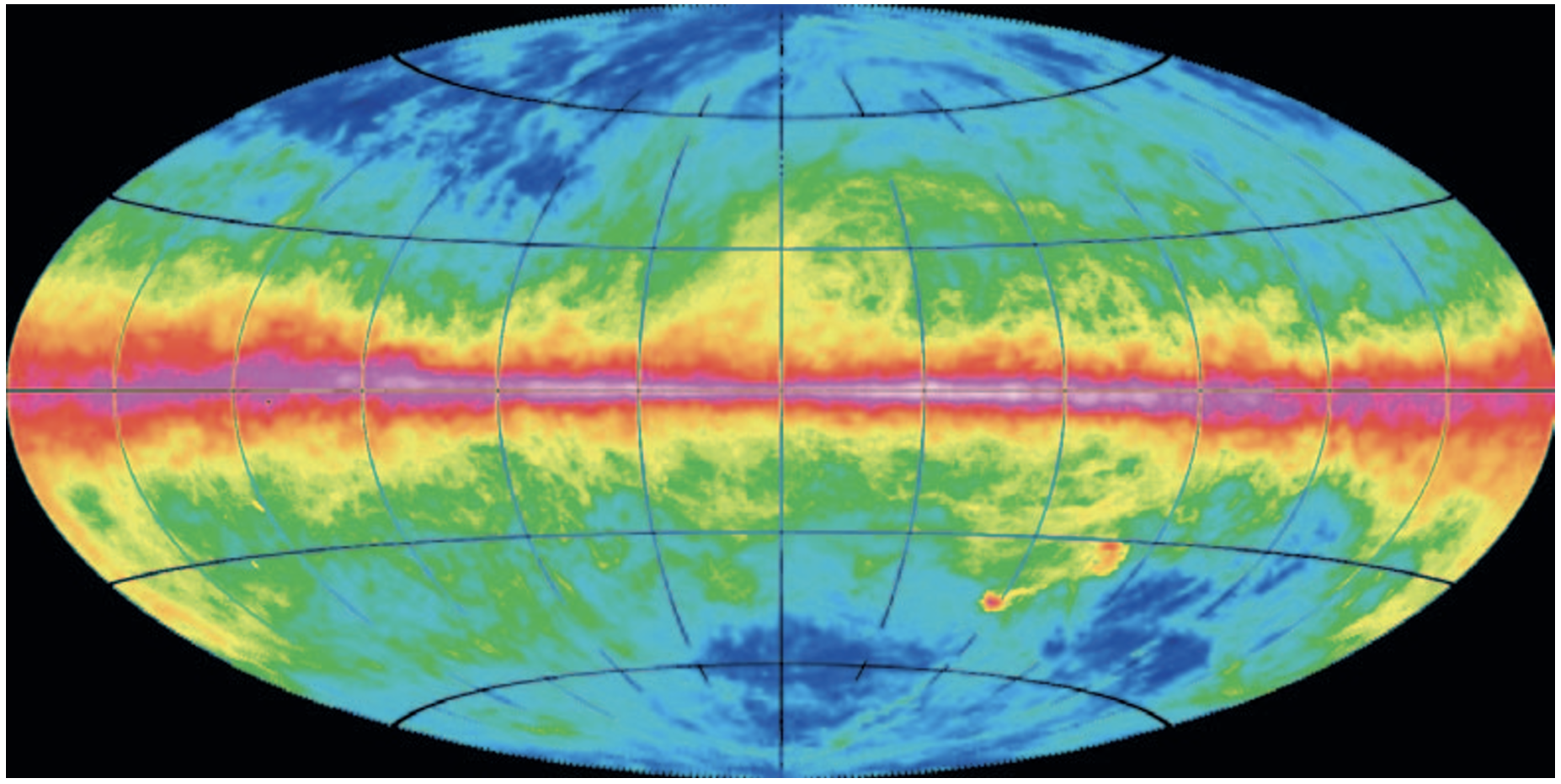
Fig. 64 H i logarithmic 21cm map of the sky from Kalberla et al. (2005) in Aitoff projection (Galactic centre in middle).#
The selection rule for transitions between hyperfine levels requires \(\Delta F = 0, \pm1\) with the exception that \(F = 0 \rightarrow 0\) is forbidden. Within the ground state of hydrogen, the nucleus consists of a single proton (\(I\) = 1/2) so either \(F = I - J = 0\) or \(F = I + J = 1\), where \(J = j\) for single electron systems. These two hyperfine states correspond to the cases in which the spins of the electron and the nucleus are parallel (\(F\) = 1) or anti-parallel (\(F\) = 0), and are separated by 0.0475 cm-1 (\(5.9 \times 10^{-6}\) eV) so transitions occur at at radio frequencies 1420 MHz (λ = 21 cm, see Fig. 63). Its existence was predicted by Hendrik van de Hulst in 1945, and first observed in 1951 by Ewen and Purcell using a ‘Horn’ antenna. A modern representation of 21cm is presented in Fig. 64 showing H I highly concentrated along the galacic plane.
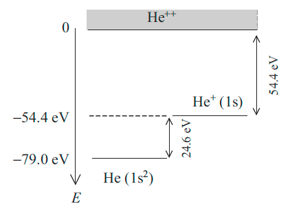
Fig. 65 Ionization energy of helium. Figure 6.2 from Mark Fox’s Atomic Physics textbook#
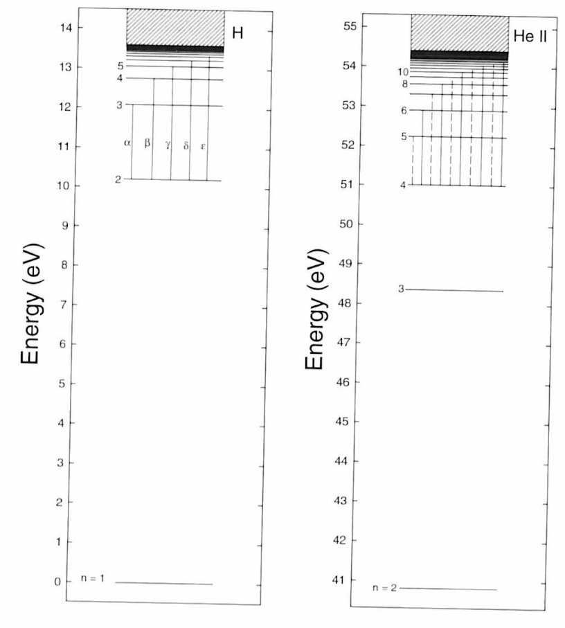
Fig. 66 Simplified energy level diagrams for hydrogen (left) and ionized helium (right). Note that the ground state of He II is not shown on this diagram (it lies at energy 0 eV). Ionized series of He II lines with lower \(n\)=4 are known as the Pickering series. Odd members (dashed) have no H i counterpart, whereas even members (solid) are coincident with H I Balmer lines. Ionized series of He II lines with lower \(n\)=3 are known as the Fowler series. Figure 2.14 from Gray & Corbally’s Stellar Spectral Classification book.#
Helium#
Fig. 65 shows the ionization energies of helium, requiring 24.6 eV to singly ionize helium, and an additional 54.4 eV (\(R^{\prime} \sim 4 R_{\infty} h c\)) to fully ionize helium since the Bohr model applies to single electron systems.
\(n_{\rm low}\) |
Discoverer |
Name |
Spectral region |
α |
β |
1 |
He Lyman |
Extreme-ultraviolet |
303Å |
256Å |
|
2 |
He Balmer |
Far-ultraviolet |
1640Å |
1215Å |
|
3 |
(Alfred) Fowler |
Fowler |
Violet-blue |
4686Å |
3203Å |
4 |
(Edward) Pickering |
Pickering |
Optical-IR |
1.01 μ m |
6560Å |
Although the energy level diagram for any hydrogen-like atom has the same form as for hydrogen, the exact spacing of the levels depends upon the atomic number, \(Z\). In the case of singly ionised helium, Eqn (13) tells us that the spacing between the energy levels is times that between the energy levels in a hydrogen atom, so the equivalent of Eqn. (16) for ionized helium is
where \(R_{He}/ch\) = 109,722 cm-1 is the Rydberg constant for helium (= 0.99986 \(R_{\infty}\)). Fig. 66 compares the energy level diagrams for hydrogen (left) and ionized Helium (right), in which the ground state of the latter is not included to allow a focus on a similar energy level range. It is apparent that energies of the principal quantum numbers of hydrogen, \(n\) below the ionization limit correspond closely to those \(2n\) for ionized helium. Consequently wavelengths of the Balmer series (e.g. Hα at 6563Å) correspond almost exactly to the even members of the He II Pickering (\(n\) = 4) series (e.g. He II 4-6 at 6560Å). This series was named after Edward Pickering (of Harvard Observatory fame) who noted their presence in ζ Puppis (O-type star) in 1896, although their identification as ionized Helium awaited Bohr’s theory. Details of spectral series of ionized He are provided in Table 2.
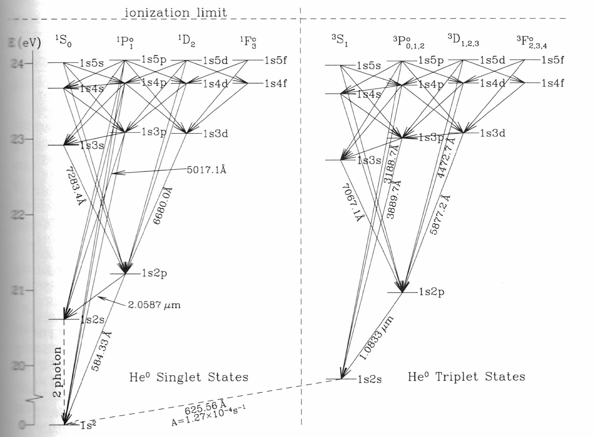
Fig. 67 Energy-level diagram for neutral helium, showing radiative decay pathways, both permitted (solid) and forbidden (dotted) lines. Figure 14.3 from Draine’s Physics of the Interstellar and Intergalactic Medium textbook.#
For multi-electron systems, such as neutral helium, one has to distinguish between quantum numbers for individual electrons within an atom and the state of the atom as a whole. Lowercase quantum numbers (\(l, s, j\)) refer to the general electron shell conflgurations, while upper case (\(L, S, J\)) refer to the sum of electron angular momenta in the outer shell, i.e.
\(L = \Sigma_i l_i\) (sum of orbital angular momenta),
\(S = \Sigma_i s_i\) (sum of spin angular momenta, integer or half-integer for odd/even numbers of electrons),
\(J = \Sigma_i j = L + S\) (vector sum of orbital and spin angular momenta).
This is known as \(LS\) or Russell-Saunders coupling and applies to light atoms and ions.
Each term is labelled by the quantum numbers \(L\) and \(S\) and is represented in the form
The total spin angular momentum \((2S+1)\) appears as a number, whereas \(L\) is a letter that follows the rule: \(S, P, D, F, G\) implies \(L = 0, 1, 2, 3, 4\), and \(p\) refers to parity[^hmnnanlHBJ][^hmnnanlHBJ]: Parity is \((-1)^{\Sigma l}\) for multi-electron systems, so is ‘odd’ for \(p, f \ldots\) orbital angular momentum (blank for ‘even’ parity, ∘ for ‘odd’ parity). The degeneracy of a term with spin \(S\) and orbital angular momentum \(L\) is \((2S+1)(2L+1)\).
A level within a term is labelled by the quantum numbers \(J\), \(L\), and \(S\) and is represented in the form
The factor \(J\) also appears as a number. The degeneracy of a level is \((2J+1)\).
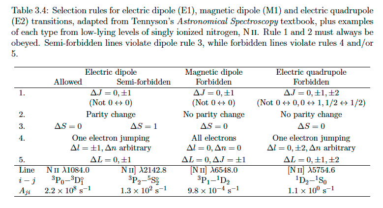
Fig. 68 Selection rules for electric dipole (E1), magnetic dipole (M1) and electric quadrupole (E2) transitions, adapted from Tennyson’s Astronomical Spectroscopy textbook, plus examples of each type from low-lying levels of single ionized nitrogen, N II. Rule 1 and 2 must always be obeyed. Semi-forbidden lines violate rule 3, while forbidden lines violate rules 4 and/or rule 5.#
For ionized helium and hydrogen, the ground state has \(L\)=0, \(S\)=1/2, \(J=1/2\) so the \(n\)=1 ground state level is 2S\(_{1/2}\) (parity is even) whereas the \(n\)=2 excited levels have \(L=0\) or 1, \(S=1/2\), \(J=1/2\) or 3/2 so 2S\(_{1/2}\) and 2P\(_{1/2,3/2}^{\circ}\). For neutral helium both electrons can occupy the innermost shell (\(1 s^2\)). \(L=S=J=0\) so the ground state term is \(^1 S_{0}\). Recombination of He+ to He0 can either occur to an excited state, or the ground state \(1 s^2 \hspace{2mm} ^1\)S0.
In the latter case, this generates \(h\nu > 24.6\)eV photons that can ionize either H0 or He0. In the former case, these will either be to states with total spin quantum number \(S = 1/2 - 1/2 = 0\) (‘anti-parallel’, known as singlets) such as \(2s \hspace{1mm} ^{1}\)S, \(2p \hspace{1mm} ^{1}\)P°, or states with \(S = 1/2 + 1/2 = 1\) (‘parallel’, known as triplets) including \(2s \hspace{1mm} ^{3}\)S, \(2p \hspace{1mm} ^{3}\)P°. The energy level diagram for He i is shown is Fig. 67. In contrast with hydrogen (and ionized helium) energies depend on both \(n\) and \(l\).
Atomic transitions can be described as ‘permitted’ if they follow electric dipole (E1) selection rules. These are presented in Fig 68 a.k.a. Table 3.4. At first they appear rather complicated but can be summarised by the following:
\(\Delta l = \pm 1\)
\(\Delta S = 0\)
\(\Delta J = 0, \pm 1\) except \(J = 0 \rightarrow 0\).
Since the emitted photon carries angular momentum, this requires at least one electron to change its angular momentum (\(\Delta l = \pm1\)), which is equivalent to the parity selection rule of even \(\leftrightarrow\) odd. The \(\Delta S = 0\) rule implies that transitions will occur only between terms of the same multiplicity.
Since \(\Delta S = 0\) for permitted transitions, so singlet helium transitions are shown to the left, and triplet helium transitions to the right of Fig. 67. Recalling \(\Delta l = 1\) for permitted transitions, cascades will take place down to the first two singlet excited states, \(1s 2s \hspace{2mm} ^{1}\)S0 or \(1s 2p \hspace{2mm} ^1 P^{\circ}_{1}\). For the latter, decays will either take place to the ground state \(1s^{2} \hspace{2mm} ^1 S_{0}\) at 584Å, or \(1s 2s \hspace{2mm} ^1\)S0 at 20581Å. The branching ratio for these lines, \(A_{584}/A_{20581} = 0.001\) so 99% will decay to λ584.
Amongst triplets, permitted lines include the fine structure transitions \(1s2s \hspace{2mm} ^{3}\)S1 and \(1s2p \hspace{2mm} ^{3}\)P\(^{\circ}_{0,1,2}\) at 10829.09, 10830.25, 10830.34Å, the strongest observable line by recombination of He+ to He0. The \(1s 2s \hspace{2mm} ^{3}\)S1 level is metastable - it can decay via spontaneous emission of a photon at 626Å to the ground state \(1s^{2} \hspace{2mm} ^{1}\)S0 but the transition is highly forbidden (\(A_{ji} = 1.3 \times 10^{-4}\) s-1, Fig. 67).
Number of |
Orbital |
Number of |
||||
\(n\) |
\(l\) |
\(m_l\) |
\(m_s\) |
orbitals |
Name |
electrons |
1 |
0 |
0 |
-1/2,+1/2 |
1 |
\(1s\) |
2 |
2 |
0 |
0 |
-1/2,+1/2 |
1 |
\(2s\) |
2 |
2 |
1 |
-1,0,+1 |
-1/2,+1/2 |
3 |
\(2p\) |
6 |
3 |
0 |
0 |
-1/2,+1/2 |
1 |
\(3s\) |
2 |
3 |
1 |
-1,0,+1 |
-1/2,+1/2 |
3 |
\(3p\) |
6 |
3 |
2 |
-2,-1,0,+1,+2 |
-1/2,+1/2 |
5 |
\(3d\) |
10 |
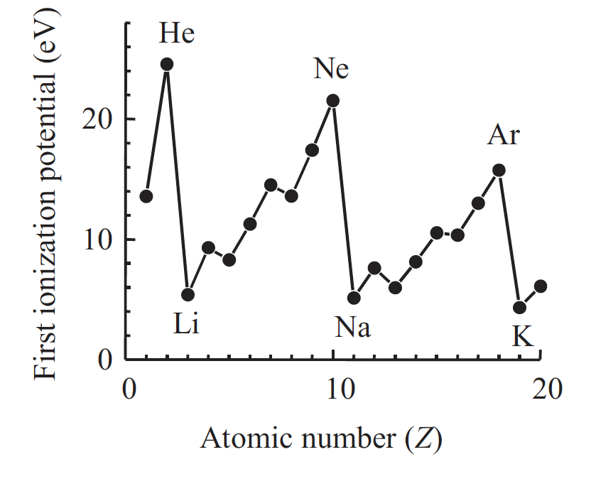
Fig. 69 First ionization potentials of elements up to Ca (in eV). Adapted from Figure 4.4 of Mark Fox’s Atomic Physics textbook.#
Complex atoms#
In general, multi-electon atoms, involve a series of shells, involving the same values of \(n\) and \(l\), with \(2(2l+1)\) degenerate levels, since magnetic quantum numbers \(m_{l}\) span \(-l, \ldots , 0, \ldots, +l\). Details of sub-shells for \(n=1-3\) are shown in Table 3 and the electronic configuration of the first 20 elements of the periodic table is shown in the final Chapter. The order of filling orbitals is:
Closed shells and sub-shells have both \(L\)=0 and \(S\)=0 so it is only necessary to consider active electrons in angular momentum calculations, i.e. those in open or partially filled shells. Elements with a single electron in the outer shell (excluding H) are known as alkali metals (Li, Na, K..), while those with fully-filled outer shells are called noble gases (He, Ne, Ar..).
Fig. 69 shows that noble gases have highly stable fully-filled shells with large ionization potentials, whereas alkali metals have one weakly bound valence electron outside fully-filled shells. Ionization potentials for all ionization stages of light elements (up to O) are shown in Fig. 70 a.k.a. Table 3.6.
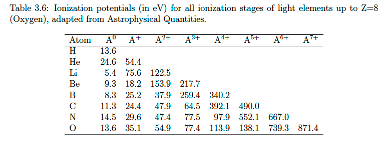
Fig. 70 Ionization potentials (in eV) for all ionization stages of light elements up to Z=8 (Oxygen), adapted from Astrophysical Quantities.#
‘Forbidden’ transitions according to magnetic dipole (M1) and electric quadrupole (E2) rules are described in Fig 68. Forbidden lines are denoted with opening ‘[’ and closing ‘]’. A transition that satisfies the E1 selection rules apart from spin is called an intercombination (in atomic spectroscopy notation) or semi-forbidden (in astrophysics notation) line (denoted with a trailing ‘]’).
Magnetic dipole transitions occur through interactions between the initial and final states of the ion. A typical magnetic moment is of order one Bohr magneton (\(\sim 10^{-20}\) cgs units) whereas a typical electric dipole moment is of order \(e a_{0} \sim 10^{-18}\) cgs units, so a typical M1 transition probability is smaller by a factor (\(10^{-20}/10^{-18})^{2} = 10^{-4}\) than an allowed E1 transition probability. For comparison, electric-quadrupole radiation is the next term in the expansion of the electromagnetic field in terms of \(2 \pi r/\lambda\) after the electric-dipole term. Here \(r\) is of order \(a_0 \sim 10^{-8}\) cm, so for optical radiation with \(\lambda \sim 5 \times 10^{-5}\) cm, \(2 \pi r/\lambda \sim 10^{-3}\). The square of this, occurs in the transition probability so this is the factor by which a typical E2 transition probability is smaller than a typical E1 one. Consequently, M1 transitions, if they occur, generally have larger transition probabilities than E2 in the optical region. Examples of each type of transition is included for singly ionized nitrogen, including Einstein \(A\) values. Here, the [N II] λ6548 M1 transition has a very low transition probability since the \(\Delta S = 0\) rule is broken.
In order to provide examples of different types of transitions, let us consider the ground state, and first excited states of the various ionization stages of oxygen (sometimes second excited states too).
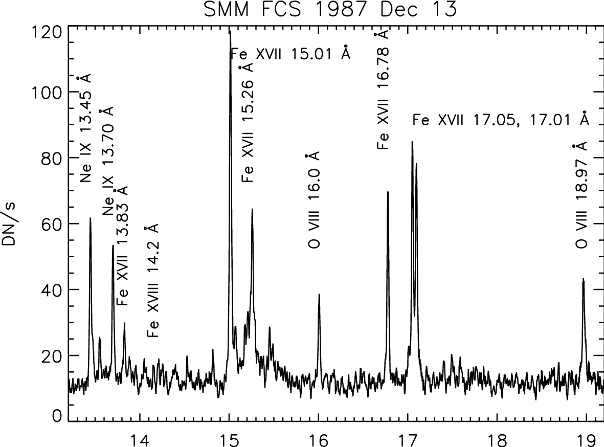
Fig. 71 Solar Maximum Mission X-ray observations of an active region of the Sun including the O VIII 18.97Å resonance line. From Del Zanna & Mason (2014).#
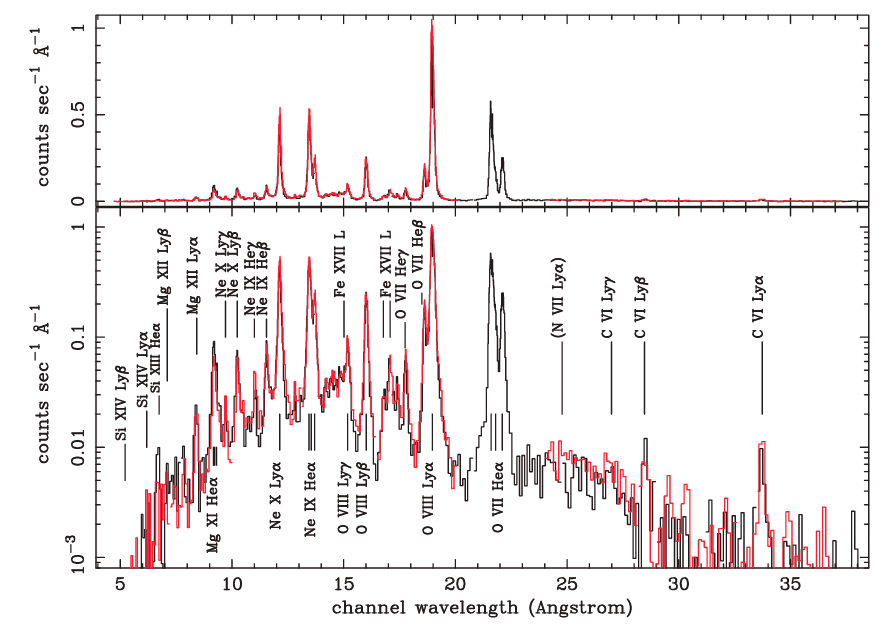
Fig. 72 Hydrogen- and helium-like emission lines of Si, Mg, Ne, O, N and C in the XMM RGS spectra of the SMC supernova remnant 1E 0102.2-7219 (linear above, logarithmic below) from Rasmussen et al. (2001).#
O VIII (H-like)#
The H-like sequence has 1 electron, with ground configuration \(1s\), so the transition connecting the O VIII ground state (\(^{2} S\)) and first excited state (\(^{2} P^{\circ}\)) is permitted and has an energy difference 82 times greater than hydrogen, a Rydberg constant of \(R_{\rm O}/hc\) = 109,733 cm\(^{-1} (= 0.99997 R_{\infty}\)), so its wavelength is at
This line is seen in X-ray observations of the Sun in Fig. 71. O VII-VIII emission lines are also observed in the SMC supernova remnant 1E 0102.2-7219 (Fig. 72), together with other hydrogen-like ions (C VI, N VII, Ne X, Mg XII, Si XIV) and He-like ions (Ne IX, Si VIII).
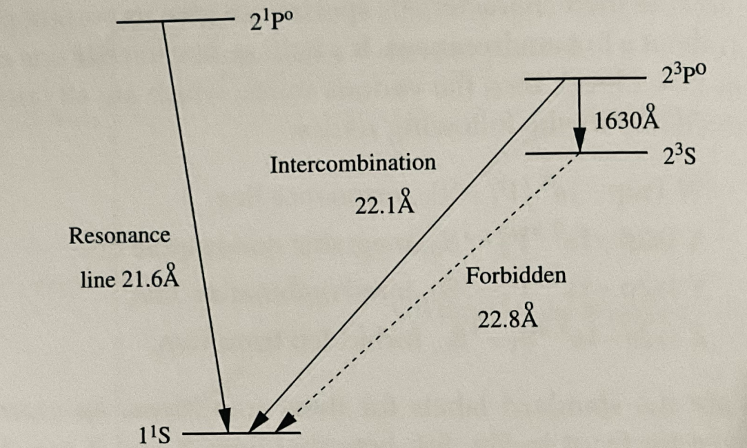
Fig. 73 Emission lines of O VII arising from \(1s 2l\) states. Fig 5.5 of Tennyson’s Astronomical Spectroscopy textbook.#
O VII (He-like)#
The He-like sequence has 2 electrons, with ground configuration \(1s^{2}\), so O VII has ground state (\(^{1} S\)) and first excited state (\(^{3} S\)), connected via a forbidden transition at 22.8Å, with the transition arising from \(^{3} P^{\circ}\) an intercombination line at 22.1Å, and the transition from \(^{1} P^{\circ}\) at 21.6Å permitted as shown in Fig. 73. The latter has the highest Einstein \(A\) coefficient (\(3.3 \times 10^{12}\) s-1), followed by the intercombination and forbidden transitions.
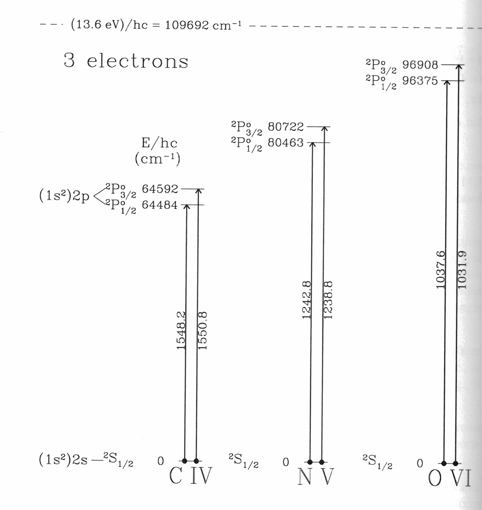
Fig. 74 Energy-level diagram of low-lying levels of O VI plus isoelectronic ions N V and C IV. Energies are shown in inverse cm (8065 cm-1 = 1 eV). The first excited state is connected to the ground state via a pair of permitted transitions (these resonance lines of C IV, N V and O VI are observed in very hot stars). From Appendix E of Draine’s Physics of the Interstellar and Intergalactic Medium textbook#
O VI (Li-like)#
The Li-like sequence has 3 electrons, with ground configuration \(1s^{2} 2s\), i.e. there is a single valence electron in its outer shell (the inner shell \(1s^{2}\) is full).The relevant energy levels for oxygen O VI, involve the ground state \(^{2} S\) and first excited state \(^{2} P^{\circ}\). This is, unusually, permitted, so transitions at 1032, 1038Å are observed in (very) high temperature star, together with isoelectronic transitions of N V and C IV (Fig. 74).
Neutral sodium also has a single valence electron in its outer shell (see Table 13) so it shares a similar energy level structure, with its ground state \(^{2}S\) and first excited state \(^{2}P^{\circ}\) connected via the 5890, 5896Å Fraunhofer D lines (responsible for the yellow-ish sodium vapour street lights).
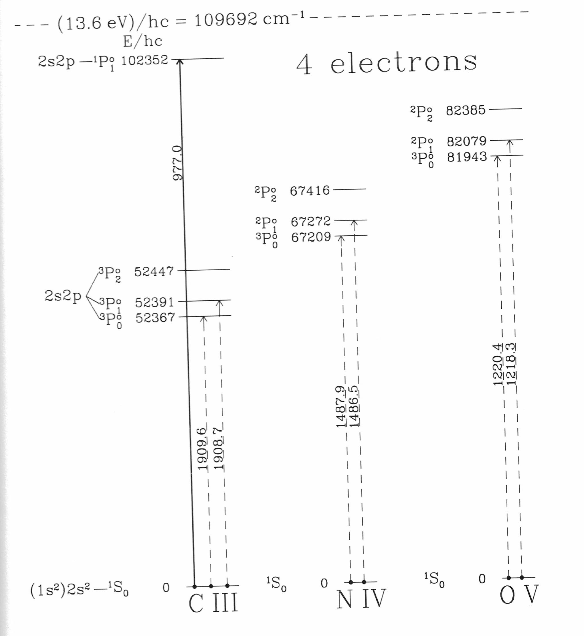
Fig. 75 Energy-level diagram of low-lying levels of O V plus isoelectronic ions N IV and C III. Energies are shown in inverse cm (8065 cm-1 = 1 eV). The first excited state is connected to the ground state via a the semi-forbidden transition from 3P\(^{\circ}_{1}\) at 1218Å and a forbidden transition from 3P\(^{\circ}_{2}\) at 1214Å (the figure includes typo for \(2S+1=3\) in upper levels of N IV and O V excited levels). From Appendix E of Draine’s Physics of the Interstellar and Intergalactic Medium textbook#
O B (Be-like)#
The Be-like sequence has 4 electrons, with ground configuration \(1s^{2} 2s^{2}\). The relevant energy levels for quadruply ionized oxygen O V involve the ground state \(^{1} S\) and first excited state \(^{3} P^{\circ}\) as shown in Fig. 75. Transitions between these are also forbidden according to electric dipole selection rules. The \(^{3} P^{\circ}_{1}\) to \(^{1} S_{0}\) transition at 1218Å is semi-forbidden (O V]) since all rules are followed aside from \(\Delta S\)=0, so has a much higher Einstein \(A\) value (\(2.3 \times 10^{3}\) s-1) than the electric quadrupole \(^{3} P^{\circ}_{2}\) to \(^{1} S_{0}\) [O V] transition at 1214Å (\(A = 0.02\) s-1). These lines are rarely observed since they lie close to Lyα in the far ultraviolet (see Chapter 4).
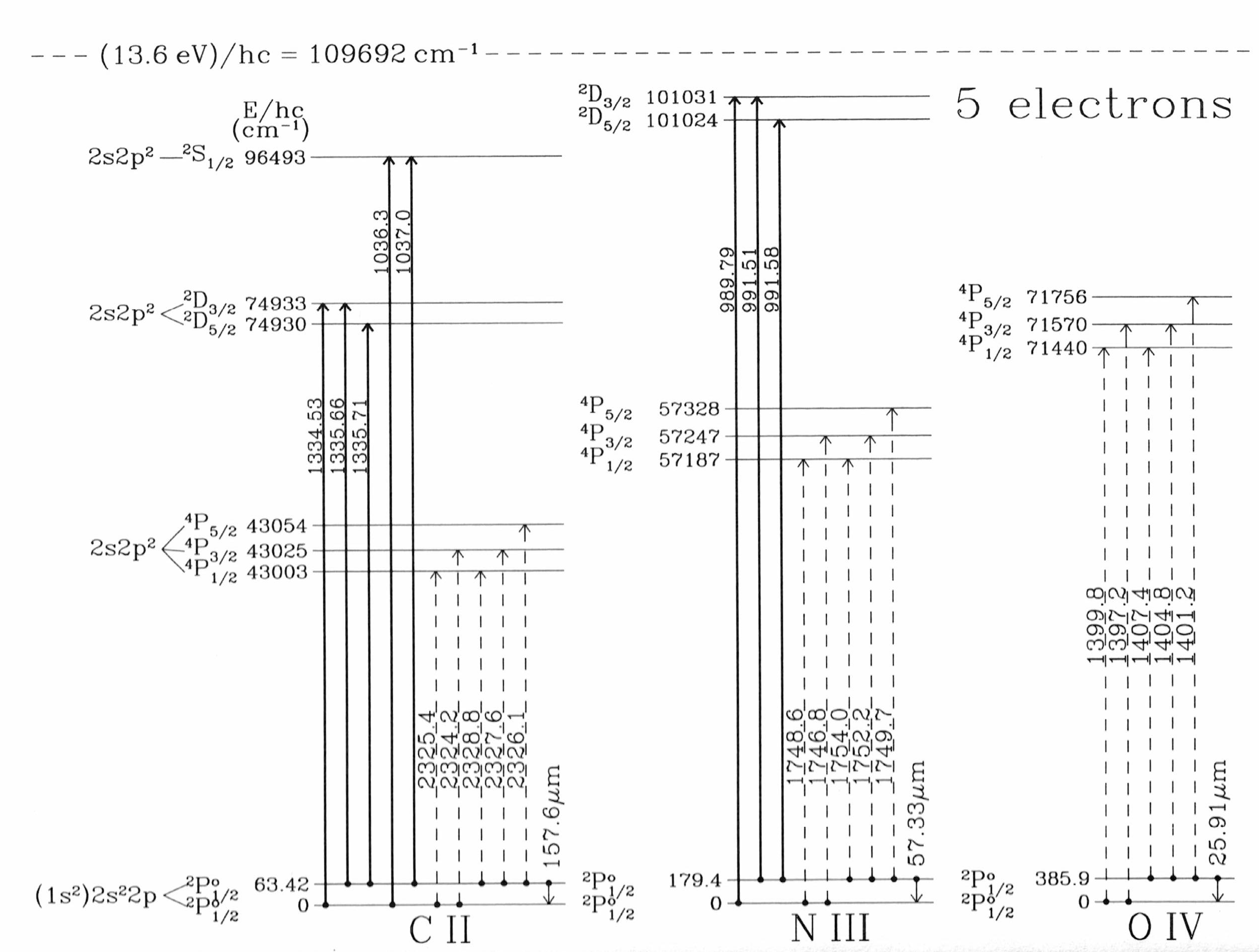
Fig. 76 Energy-level diagram of low-lying levels of O IV plus isoelectronic ions N III and C II. Energies are shown in inverse cm (8065 cm-1 = 1 eV). The first excited state is connected to the ground state via a forbidden transition, and a fine structure forbidden transition within the ground state lies at 25.9μm. From Appendix E of Draine’s Physics of the Interstellar and Intergalactic Medium textbook.#
O IV (B-like)#
The B-like sequence has 5 electrons, with ground configuration \(1s^{2} 2s^{2} 2p\). The relevant energy levels for triply ionized oxygen O IV involve the ground state \(^{2} P^{\circ}\) and first excited state \(^4 P\). Transitions between these are also forbidden, with wavelengths close to 1400Å in the far ultraviolet (there are multiple components within this multiplet). An energy level diagram for O IV (plus N III and C II) is presented in Fig. 76 and also shows a forbidden fine-structure transition within the ground state at [O IV] 25.9μm.
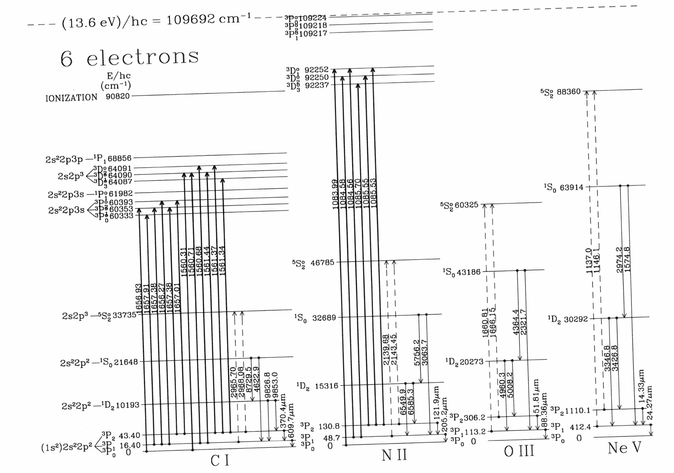
Fig. 77 Energy-level diagram for lowest terms of C I, N II, O III and Ne V. Energies are shown in inverse cm (8065 cm-1 = 1 eV). Splitting of the ground \(^{3}P\) term has been exaggerated for clarity. Transitions within the ground state of [O iii] involve 51.8μm between \(J=2,1\) and 88.4μm between \(J=1,0\). From Appendix E of Draine’s Physics of the Interstellar and Intergalactic Medium textbook.#
O III (C-like)#
The C-like sequence has 6 electrons, with ground configuration \(1s^{2} 2s^{2} 2p^{2}\). The relevant energy levels for doubly ionized oxygen are shown in Fig. 77 (together with N II which has an identical shell structure). The ground state is a \(^{3} P\) term, whereas the first excited state is a \(^{1} D\) term, so this transition too is forbidden by E1 rules, but the \(^{3} P_{2} - ^1 D_{2}\) and \(^{3} P_{1} - ^1 D_{2}\) transitions satisfies the M1 (and E2) rules on \(\Delta J\) (not \(\Delta S\)) = 0). These are the green 5007, 4959Å lines. The transition probability ratio of the λ5007 to the λ4959 lines is 3.01 according to theory, implying an intensity ratio of 2.98 (Storey & Zeippen 2000) so a ratio of 3:1 is usually adopted. The transition between \(^{3} P_{0} - ^1 D_{2}\) at λ4931 is not shown because it is only satisfies the E2 rules, so has a tiny Einstein \(A\) value (\(2.4 \times 10^{-6}\) s-1).
The second excited state (\(^1 S\) term) is connected to the ground state and first excited states through forbidden transitions, the latter at 4363Å. This, together with the strong green lines will also be discussed in Chapter 5 in the context of electron temperatures. Fig. 77 also shows transitions within the ground state \(^{3} P\) term. These are fine-structure lines at 51.2μm (J = 2 to 1) and 88.4μm (J = 1 to 0), also commonly observed in ionized nebulae.
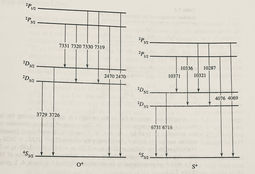
Fig. 78 Energy-level diagrams of low lying transitions of O II and S II. Figure 5.7 from Kwok’s Physics and Chemistry of the ISM textbook.#
O II (N-like)#
The N-like sequence has 7 electrons, with ground configuration \(1s^{2} 2s^{2} 2p^{3}\). The relevant energy levels of singly ionized oxygen are shown in Fig. 78 (together with S ii which has the same outer shell structure). The ground state is a \(^{4} S^{\circ}\) term, whereas the first excited state is a \(^{2} D^{\circ}\) term so this transition is forbidden by E1 rules, but satisfies the M1 (and E2) rules on parity and \(\Delta J\) (not \(\Delta S\) = 0). This is the violet doublet at 3727, 3729Å, which is a strong emission line in many nebulae and as we shall discuss in Chapter 5 is a sensitive diagnostic of electron density in such environments.
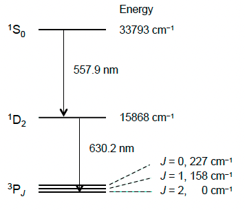
Fig. 79 Lowest levels of atomic oxygen showing forbidden transitions responsible for the green (5577Å) and red (6300Å) auroral lines (splitting within the ground state is exaggerated for clarity). Figure 12.4 of Mark Fox’s Atomic Physics textbook.#
O I #
The O I sequence has 8 electrons, with ground configuration \(1s^{2} 2s^{2} 2p^{4}\), resulting in the terms of four equivalent \(p\) electrons, namely 3P, 1D and 1S. The ground state is the \(^{3} P\) term and the first excited state is the \(^{1} D_2\) term, so this transition is forbidden by electric dipole rules, but the \(^{3} P_{2} - ^1 D_{2}\) transition satisfies the M1 and E2 rules on electron jumps, parity, and \(\Delta J\) (not \(\Delta S\)) =0). This is the red auroral line at 6300Å. The transition between the first ( \(^1 D_{2}\)) and second excited states (\(^1 S_{0}\)) is also forbidden, since no electron jumps shell, parity is unchanged and \(\Delta J = 2\) but these are permitted for E2. This is the green auroral line at 5577Å. These can also be seen in the sky spectrum shown in Fig. 48.
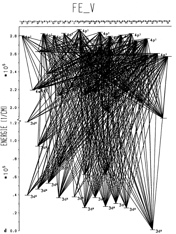
Fig. 80 Comprehensive energy-level diagram for Fe V. Energies are shown in inverse cm (8065 cm-1 = 1 eV). Figure 2 from Pauldrach et al. (1994).#
Here, we have discussed the ground and low level states of different ionization stages of oxygen (the most abundant element after H and He). This exercise explains why we need to consider forbidden as well as permitted lines since the first and second excited levels are usually the highest populated levels after the ground state (recall Eqn. (19)). We have also shown that the structure of most atoms is much more complex than hydrogen or helium. To illustrate this further, Fig 80 shows the Grotrian diagram for Fe V.
Radiative transitions#
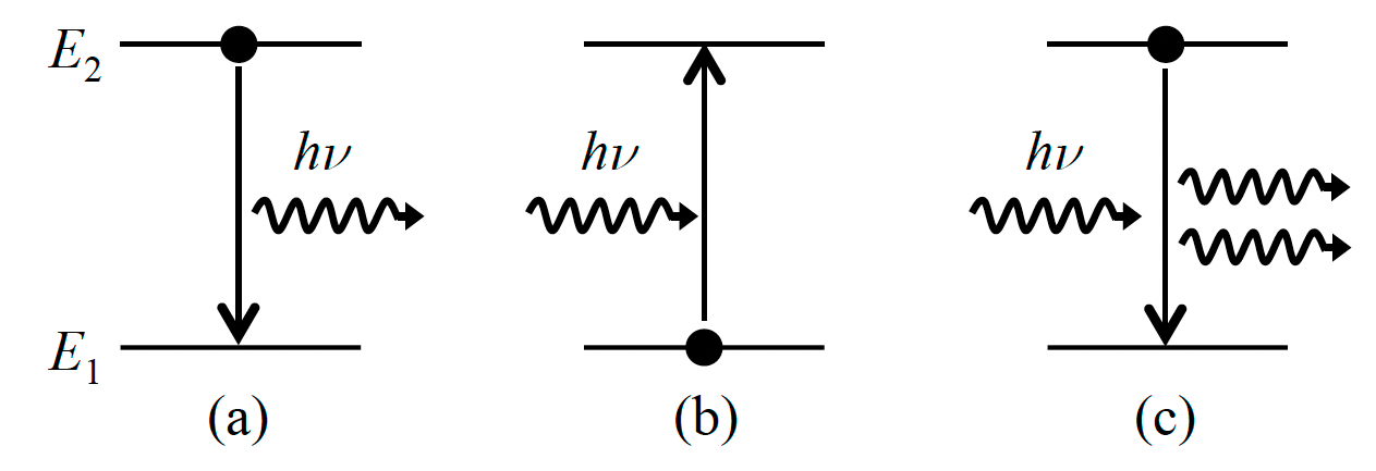
Fig. 81 Different types of transitions between levels of an atom: (a) spontaneous emission; (b) absorption; (c) stimulated emission. Figure 9.1 from Mark Fox’s Atomic Physics textbook.#
Let us now turn to radiative transitions, and consider an idealised two level atom, in which level 1 is the ground state and level 2 the excited state. We have previously introduced spontaneous emission earlier in this chapter, involving the Einstein \(A\) coefficient. This is illustrated in Fig. 81(a).
If the atom starts in the lower level 1, it can be induced to make a transition to the upper level 2, by absorbing a photon of the same energy. This is illustrated in Fig. 81(b). Einstein realised that a third process, called stimulated emission, is requires for a consistent solution to the problem of interactions between a gas of atoms and blackbody radiation in thermal equilibrium. Stimulated emission is the reverse of absorption, as illustrated in Fig. 81(c).
An atom in level 2 drops to 1 stimulated by photons with energy \(h \nu = E_{2} - E_{1}\). In the case of a gas irradiated by blackbody radiation, the three types of transition shown in Fig. 81 can be expressed as follows.
Spontaneous emission,
stimulated emission,
and absorption
These equations define the Einstein A and B coefficients, the latter giving the probabilities for the stimulated processes. Rates for stimulated transitions also scale with the number of atoms and radiation field energy density. – Some textbooks (Rybicki & Lightman’s Radiative Processes in Astrophysics) use mean intensity \(J_{\nu}\) in these expressions, differing Einstein \(B\) coefficients differing by a factor of \(4\pi/c\) \(\rho_{\nu}\)– In equilibrium the rate of upward transitions must balance precisely the rate of downward transitions:
so
where in thermodynamic equilibrium the ratio of \(N_{1}\) to \(N_{2}\) is
where \(g_{2}\) and \(g_{1}\) are statistical weights (degeneracies) of levels 2 and 1, and \(k\) is Boltzmann’s constant. Consequently the radiation field can be expressed in terms of Einstein coefficients
In thermodynamic equilibrium, the specific energy density \(\rho_{\nu} = (4\pi/c) B_{\nu}\) where \(B_{\nu}\) is the Planck formula
so
and
i.e, the Einstein \(A\) and \(B\) coefficients are intimately linked. This approach can be generalized to more than the two level case, adopting the principle of detailed balance which connects any microscopic process and its inverse (here absorption and emission).
If we can measure the radiative lifetime of a transition, we can determine \(A_{ul}\), and in turn determine the Einstein \(B\) coefficients from Eqns (20)-(21). Finally, intrinsic line strengths can also be characterized in terms of (dimensionless) oscillator strengths, denoted \(f_{21}\), which are commonly used when discussing stellar absorption lines (more on this in PHY305). Oscillator strengths are linked to the Einstein \(A\) coefficient via:
for \(\lambda_{12}\) expressed in Å. By way of example, oscillator strengths for prominent hydrogen lines are shown in Table 4
Line |
Transition |
\(f_{12}\) |
\(A_{ji}\) (s -1 ) |
Ly α |
\(1s-2p\) |
0.416 |
\(6.3 \times 10^{8}\) |
Ly β |
\(1s-3p\) |
0.079 |
\(1.7 \times 10^{8}\) |
Ly γ |
\(1s-4p\) |
0.029 |
\(6.8 \times 10^{7}\) |
Ly δ |
\(1s-5p\) |
0.014 |
\(3.4 \times 10^{7}\) |
Ly ε |
\(1s-6p\) |
0.008 |
\(2.0 \times 10^{7}\) |
Ly ζ |
\(1s-7p\) |
0.004 |
\(1.1 \times 10^{7}\) |
Ly η |
\(1s-8p\) |
0.003 |
\(8.2 \times 10^{6}\) |
Collisional transitions#
Electron collisions with ions may result in excitation to excited levels. Unlike radiative transitions, collisional transitions are not restricted by parity rules, so electron-ion collisions are the primary mechanism for exciting low-lying transitions of the same parity, where radiative transitions have extremely small probabilities. The energies of levels that can be excited are related to the kinetic temperatures of the free electrons, known as the excitation temperatures (\(\chi = kT\)).
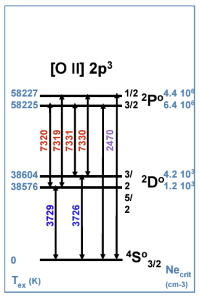
Fig. 82 Excitation temperatures for low lying levels of [O II]#
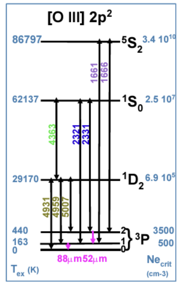
Fig. 83 Excitation temperatures for low lying levels of [O III]#
Excitation temperatures for low lying levels of O ii and O iii are shown in Fig. 82 and Fig. 83. For example, [O iii] λ5007 arises from a level 2.51 eV above the ground state, so its excitation temperature is \(2.9 \times 10^{4}\) K, conditions similar to those within ionized nebulae. Excited levels of H and He have much higher excitation potentials so are rarely collisionally excited. For example, the \(n=2\) level of hydrogen sits 10.2 eV above the ground state so has an excitation temperature of \(1.2 \times 10^{5}\) K, while the upper level of the neutral He λ584 line has an excitation temperature of \(2.5 \times 10^{5}\) K. For higher temperature-density sources, such as the solar corona (\(T_{e} \sim 10^{6-7}\) K), more highly ionized species come into play (e.g. O vii-viii),
For our idealised two level atom, the collisional excitation rate per unit volume per unit time is
where
in units of cubic cm per second for excitation energy \(\chi_{12}\) where \(\Omega_{12}\) is the collision strength, \(E_2\) is the energy of the incident electron and
is the effective collision strength averaged over the Maxwellian distribution of electron velocities. At high densities, the population distribution is dominated by collisions and the principle of detailed balance requires that the excitation rate from lower level 1 to upper level 2 is exactly balanced by the de-excitation from 2 to 1,
so recalling the Boltzmann equation Eqn (19), the de-excitation collision rate
Collisional and radiative transitions#
We can combine radiative and collisional transitions for our idealised two level atom in equilibrium as follows:
In regions where the radiation field is weak, the stimulated terms are unimportant so the equation of statistical equilibrium reduces to
At high densities this reverts to the Boltzmann distribution (Eqn (24)). Permitted transitions in the UV and optical have \(A_{21} \geq 10^{8}\) s-1 while collisional de-excitation coefficients are \(C_{21} \leq 10^{-18}\) cm3 s-1 so if the density is \(n_{e} \leq 10^{12}\) cm-3 then \(C_{21} n_{e} \ll A_{21}\) so we can make the coronal approximation
i.e. the dominant processes are collisional excitation and spontaneous radiative de-excitation, so relative populations are not given by the Boltzmann distribution. This is known as the coronal approximation since it applies to the upper chromosphere and corona of the Sun.
We can now determine the power, or emissivity \(\epsilon_{21}\) of the transition from level 2 to level 1, per unit volume (equivalent to the cooling rate). The line luminosity is
where \(V\) is the volume of the emitting material. Line intensities are integrated emissivities adjusted for the inverse square law at a distance \(d\)
and has units erg cm-2 s-1.
At high densities, \(\epsilon_{21} = N_{2} A_{21} h \nu_{21}\) or recalling the Boltzmann formula (Boltzmann) \(\epsilon_{21} = N_{1} \frac {g_2}{g_1} \exp (-\chi_{12}/k T_{e}) A_{21} h \nu_{21}\), so the cooling rate depends on the Einstein \(A\) coefficient. In contrast, at low densities (coronal approximation) the emissivity becomes \(\epsilon_{21} = h \nu_{21} N_{1} C_{12} n_{e}\), in which case the cooling rate depends on the collision rate instead of the spontaneous emission coefficient.
The approach followed depends on whether the emitting material has an electron density above or below the critical density. For a two level atom the critical density, \(n_{c}\), is defined as the density at which the collisional de-excitation rate equals the spontaneous decay rate, i.e. \(A_{21} = C_{21} n_{c}\). For \(n_{e} \ll n_{c}\) collisional de-excitation is unimportant, whereas for \(n_{e} \gg n_{c}\) level populations are set by the collisional coefficients. We will return to the critical density in Chapter 5.
As well as considering radiative and collisional excitation and de-excitation rates for multiple levels, in reality ionization and recombination processes (collisional or radiative) also come into play, but these too will be deferred until our discussion of ionized nebulae in Chapter 5. Since we focus in this course largely on emission, rather than absorption, processes, there are three flavours in thermal plasmas:
Bound-bound transitions, where the emitting electron makes a transition from one bound state to another, with the difference in energy carried away by one or two photons,
Free-bound transitions, where the emitting electron is initially free, but is captured into a bound state, with emission of a continuum photon,
Free-free transitions, where the emitting electron is inelastially scattered from one free state to another, with emission of a continuum photon (Bremsstrahlung radiation).
Example 3.1
A proton and electron recombine to form atomic hydrogen in its \(4p\) state. At what wavelengths will recombination lines be subsequently observed? How would the observed emissions differ if the atom had recombined into the \(4s\) level?
Selection rules for permitted transitions include \(\Delta l = \pm 1\) and \(\Delta n\) = any, so series include direct recombinations: \(4p-3s, 4p-3d\) (Pα), \(4p-2s\) (Hβ), \(4p-1s\) (Lyγ) and indirect recombinations: \(3s-2p, 3d-2p\) (Hα) plus \(2p-1s\) (Lyα). Starting from the \(4s\) level, \(4s-3p\) (Pα) will lead to \(3p-1s\) (Lyβ) but not Lyγ.
Example 3.2
An emission line of He II is observed at 1640Å. Which transitions does this line correspond to?
Rearranging Eqn (17), \((1/n^{2} - 1/m^{2}) = 1/(2^{2} \times 109722 \times 1640 \times 10^{-8}) = 0.1389\), recalling units of cm for Rydberg constants, so \(n\) = 2, \(m\) = 3. 1640 line is the He+ equivalent of Hα (1/4 wavelength since 22 energy difference).
Example 3.3
The symbol for a particular level is 4F\(^{\circ}_{7/2}\). What are the values of \(L, S\) and \(J\) for this level? What is its degeneracy? What are the other levels of this term?
\(L\)=3, \(S=\frac{3}{2}\) and \(J=\frac{7}{2}\). Degeneracy is \((2J+1)=8\). Possible levels are given by \(| L-S | < J < L+S\) i.e. \(\frac{3}{2}, \frac{5}{2}, \frac{7}{2}, \frac{9}{2}\), i.e. three additional levels within the term.
Example 3.4
Give an expression for the energy levels of H-like atoms of nuclear charge \(Z\) in term of R∞. Obtain the energy (in eV) of the Lyα transition of H-like nitrogen N VII. From what astronomical environment would such transitions occur and how might they be observed?
From Eqn (14), \(E_{n} \sim -\frac{Z^{2} (R_{\infty} hc)}{n^{2}}\) where \(R_{\infty} hc\) = 13.606 eV. For \(Z=7\), the Lyα transition involves \(n\) = 1 and \(n\) = 2, so \(\Delta E_{12} = 500\) eV (0.5 keV) or 24.8Å. This lies in the X-ray part of the electromagnetic spectrum and has an excitation temperature (\(T\sim E/k\)) of 6 million Kelvin, so requires very hot plasma (e.g. solar corona, SNR).
Example 3.5
The transition frequency between quantum numbers \(n_1\) and \(n_2\) of atomic hydrogen is provided in Eqn. (15). In which part of the electromagnetic spectrum does the line transition between the \(n_1\)=76 and \(n_2\)=77 orbitals occur?
\(\nu_{76,77} = (1.097 \times 10^{5}) \times (2.998 \times 10^{10}) (1/76^2 - 1/77^2) = 1.47 \times 10^{10}\) Hz or \(\lambda_{76,77} = 0.020\) m or 2cm (radio).