Chapter 5: Ionized nebulae

A physical understanding of stellar spectroscopy awaits a discussion of radiative transfer in PHY305, but having introduced relevant aspects of atomic physics, line formation (radiative and collisional) plus interstellar extinction we are now able to interpret spectroscopic observations of ionized nebulae, which will also be the focus of the laboratory exercise. Further reading:

• Physics of the Interstellar Medium. John Dyson, & David Wiliams, IoP Graduate Series in Astronomy

• Astrophysics of Gaseous Nebulae and Active Galactic Nuclei, Donald Osterbrock, & Gary Ferland, University Science Books

• Atoms, stars and nebulae, Lawrence Aller, Cambridge

Types of nebulae

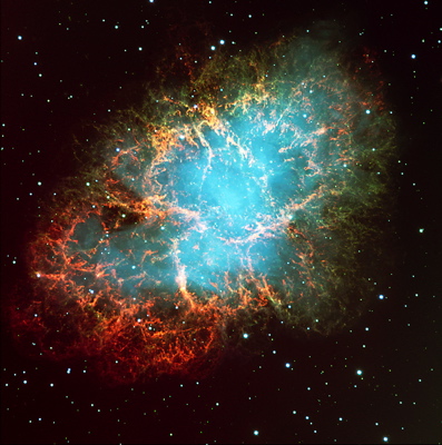
Fig. 92 Image of Crab nebula (M1)

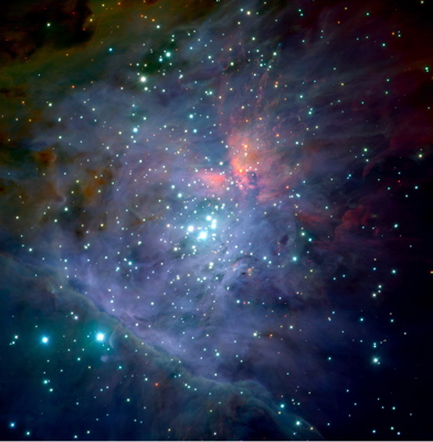
Fig. 93 Image of Orion nebula (M42)

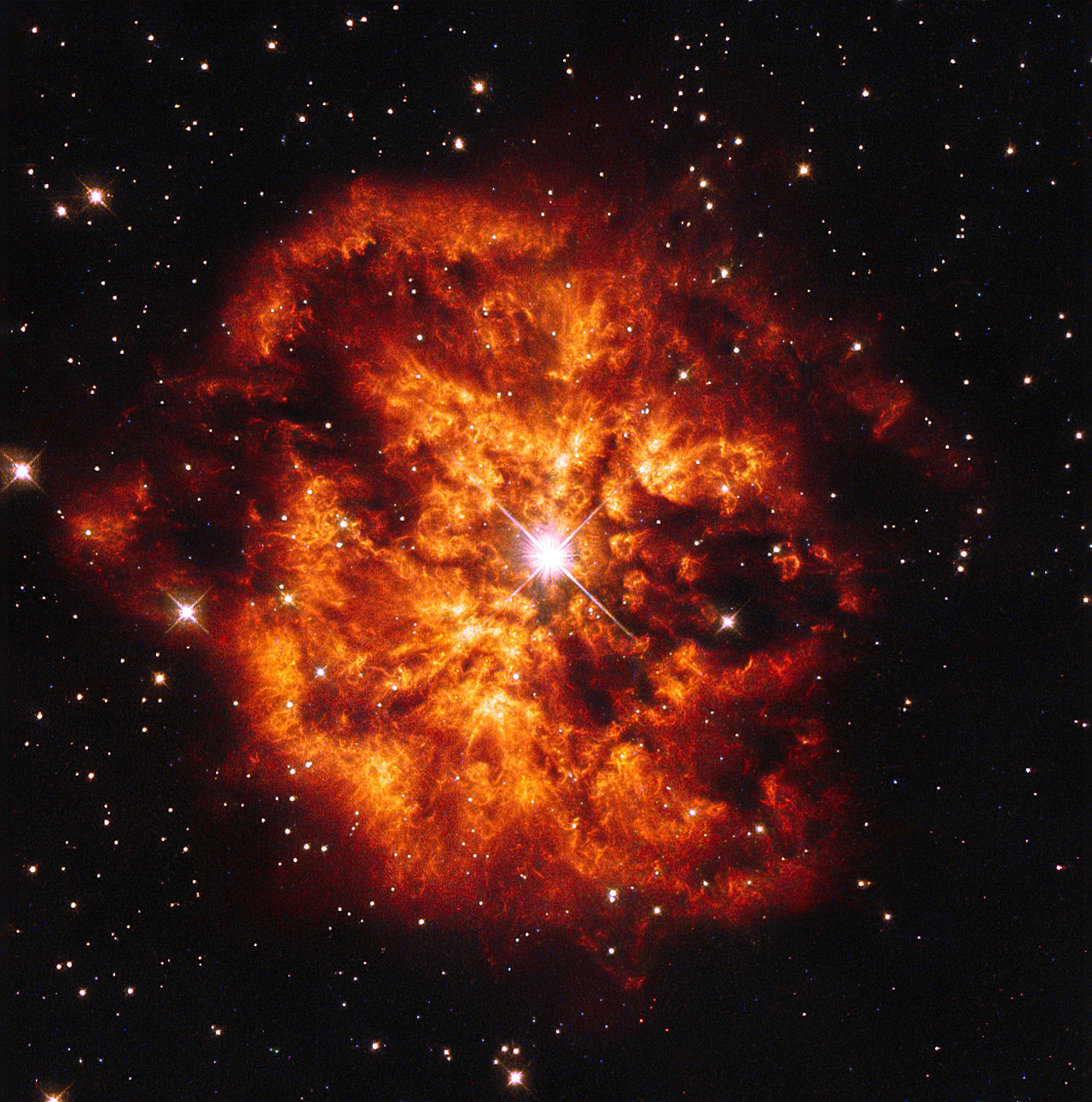
Fig. 94 Image of M1-67 nebula

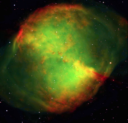
Fig. 95 Image of Dumbbell nebula (M27)

There are a broad range of nebulae in astrophysics. Examples include the Crab nebula (Fig. 92), the Orion nebula (Fig. 93), the M1-67 nebula (Fig. 94), and the Dumbbell nebula (Fig. 95). All involve extended regions of gas and/or dust, but involve very different physical phenomena. Three of these were recorded by Charles Messier, whose catalogue was devised in an attempt to avoid confusion with comets. Nebulae (excluding external galaxies and star clusters which were also included in the Messier catalogue) can be categorized into several types:

• *H II regions These nebulae arise when hot, luminous stars in young stellar nurseries (photo)ionize gas left over from the star formation process. An example is the Onion Nebula in which several massive stars in a compact star cluster are responsible for this H II region. These span a range of sizes, parsec scale for compact H II regions such as Orion, tens of parsecs for Giant H II regions (e.g. Carina Nebula in the Southern sky) and hundreds of parsec for the Tarantula Nebula in the LMC (supergiant H II region which is host to 1000 OB stars.

• Planetary nebulae These nebulae are (photo)ionized by an evolved low mass star which has been stripped of its hydrogen-rich envelope in the AGB phase to reveal a bare hot core (e.g. Horsehead nebula). Consequently the physical mechanism responsible for PNe is the same as some H II regions (gas ionized by hot central star) but PNe are associated with old stellar populations, whereas H II regions are young.

• Supernova remnants These nebulae are shock ionized as the rapidly expanding supernova encounters material either thrown off from its progenitor or the surrounding ISM. The star responsible for the Crab nebula SNR exploded in 1054 and at its heart is a rapidly rotating neutron star (pulsar). SNR remain bright for tens of thousands of years (e.g. Vela).

• Ejecta nebulae Ejecta nebula are photo-ionized by massive stars which strip away their outer hydrogen-rich layers at the end of their (brief) lives, revealing a hot blue star, and include M1-67 associated with the Wolf-Rayet star WR124

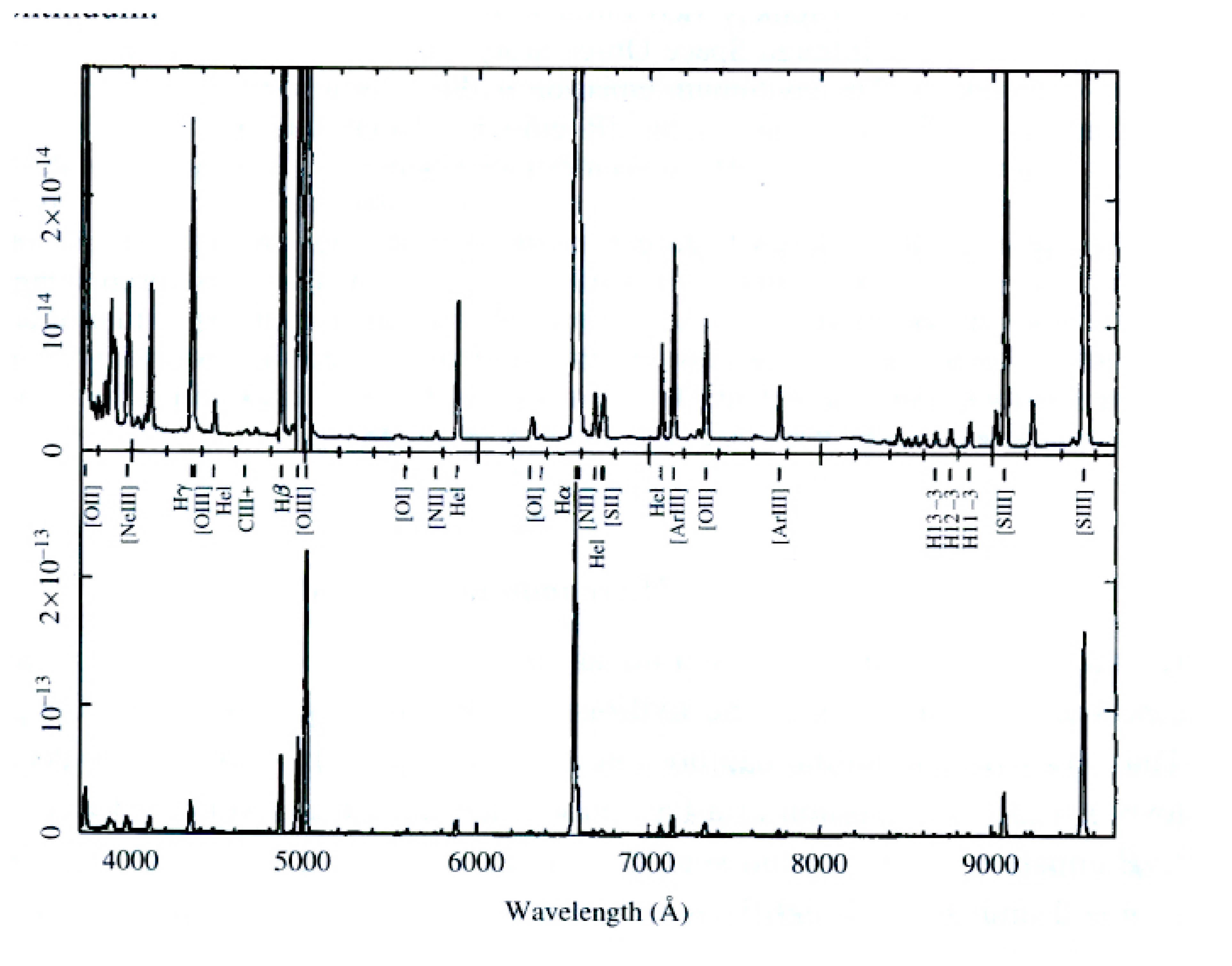
Fig. 96 Visual spectrum of the Orion nebula, showing strong (lower panel) and weak (upper panel) nebular emission lines. Baldwin et al. (1991)

Spectroscopy of ionized nebulae

In this course we shall focus on spectroscopy of (photo)ionized nebulae, predominantly H II regions. The visual spectrum of the Orion Nebula is presented in Fig. 96. The lower panel reveals strong permitted emission lines due to hydrogen (H\(\alpha, \beta, \gamma\)) but forbidden lines of metals are also prominent, including [O III] \(\lambda\lambda\)4959,5007, [S III] \(\lambda\lambda\)9069,9532. In the upper panel weaker lines can be seen including permitted (He i λ5876, λ7065) and forbidden ([O II] \(\lambda\lambda\)3727,3729, [Ar III] λ7751). Higher spectral resolution (echelle) observations of the Orion nebula are discussed in Esteban et al. (2004) (recall Fig. 61).

The optical spectra of PNe are broadly similar to those of H, ii regions, as shown in Fig. 97, although the ionizing stars are usually much hotter (albeit less luminous), so higher ionization lines are observed (e.g. He ii λ4686, [Ar IV] λ4711, 4740). Forbidden [O III] \(\lambda\lambda\)4959,5007 lines are exceptionally strong in NGC7009, whereas permitted O ii lines (zoom) are very weak. Although we shall primarily focus on optical spectroscopy, ionized nebulae also exhibit strong permitted (hydrogen) and forbidden (metal fine-structure) lines in the infrared, as shown in Fig. 98.

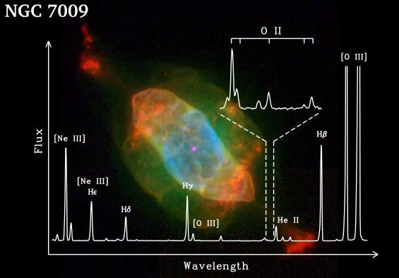
Fig. 97 Visual spectrum of NGC7009 nebula, superimposed on an image of this PNe. Compare the strengths of forbidden [O  III] \(\lambda\lambda\)4959,5007 (off scale) to the zoomed in view of permitted O  ii lines, adjacent to He  ii λ4686.

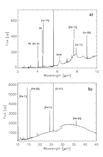
Fig. 98 Mid-infrared spectrum of the PNe NGC7027 with ISO/SWS showing strong permitted (e.g. Brα) and forbidden (e.g. [Ne III] 15.5μm, [O IV] 25.9μm) lines. The continuum represents warm dust emission (PAH stands for Polycyclic Aromatic Hydrocarbons). Ref: Bernard-Salas et al. (2001).

Pure hydrogen nebulae

In the case of a pure hydrogen nebula, photoionization arises when photons with energy \(h\nu \geq \chi_{H}\) liberate the electron from the proton (\(\chi_{H}\) = 13.6 eV). Any excess energy goes into the kinetic energy of the electron. The strong Coulomb interaction between protons (positively charged) and electrons (negatively charged) produces the inverse process, namely recombination. The energy of the recombined H atom is the sum of the kinetic energy of the recombining electron plus the binding energy of the electron in the energy level to which it recombines (\(\chi_{H}/n^2\)). Photons are emitted as the electron cascades down towards the ground state \(n\)=1.

In a nebula composed of electrons, protons and neutral atoms the gas is continuously being fed energy via photoionization of atoms. These are injected via the kinetic energy of electrons, which exhibit a Maxwellian velocity distribution, so the gas temperature is referred to as the electron temperature \(T_{e}\).

Recombination rate

In equilibrium there is a balance between photoionizations and recombinations. When considering the ionization balance, one needs to compare recombination and ionization rates per unit volume of gas. Recombination may occur into any level of quantum number \(n\) at a rate of \(\alpha_n\). The recombination rate scales with the product of the electron number density, \(n_{e}\) and proton number density \(n_{p}\) and is a function of \(T_{e}\) since the rate at which a proton encounters an electron depends on the electron velocity distribution. Consequently the volume recombination rate into level \(n\) is

\[\frac{dN_{n}}{dt} = n_{e} n_{p} \alpha_n (T_{e}) = n_{e}^{2} \alpha_n(T_{e})\]

since \(n_{e} = n_{p}\) in a pure H nebula.

We need to the total recombination rate into all level. If an electron with kinetic energy \(E (\sim kT_{e}\)) recombines into level \(n\), it will emit a photon of energy

\[h \nu = \frac{\chi_{\rm H}}{n^2} + E.\]

where \(\chi_{H}/n^{2}\) is the binding energy of level \(nl\). Therefore when recombination takes place directly to the ground state \(n\)=1, a photon will be emitted that can ionize hydrogen. i.e. ground-state recombinations are assumed to be balanced by an immediate ionization. For H II regions it is reasonable to assuming that the total recombination rate \(dN_{R}/dt\) includes recombination into all levels \(n\geq2\)

\[\frac{dN_{R}}{dt} = \Sigma_{n=2} \frac{dN_{n}}{dt} = n_{e}^{2} \alpha_B (T_{e}).\]

A numerical approximation of the recombination coefficient

(33)\[\alpha_{B} (T_{e}) = 2 \times 10^{-10} T_{e}^{-3/4} \]

in units of cubic cm per second. The ‘B’ in this expression signifies Case B recombination theory (only recombinations to \(n\geq2\) are considered) as opposed to Case A recombination theory (recombinations to all levels are considered), terminology first introduced by Baker & Menzel (1938). Case A applies to shock-heated regions where H is collisionally ionized are typically very hot (\(\geq 10^{6}\) K) and contain very little neutral hydrogen so only a negligible fraction of photons emitted in recombinations to \(n\)=1 will photoionize H within the nebula.

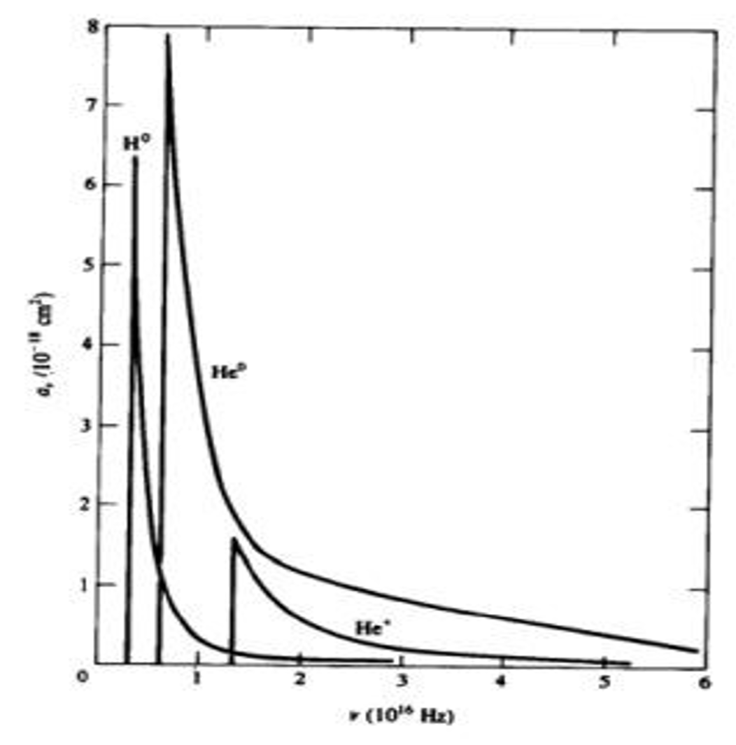
Fig. 99 Photoionization absorption cross-sections, \(\sigma_{\nu}\), of H⁰ (threshold 912Å), He⁰ (threshold 504Å) and He⁺ (threshold 228Å) ions. Fig 2.2 from Osterbrock & Ferland’s AGN² textbook.

Ionization rate

Lifetimes of excited states of H are very short. For example, \(A_{ul} = 6\times 10^{6}\) s^-1 for Hα from Figure 58, so \(\tau (H\alpha) = 1/A_{ul} = 0.17\) ms. Therefore the probability of ionizing a H atom in an excited state is negligible. Consequently, when calculating the ionization rate we may assume all the H atoms lie in the ground state \(n\) = 1. If the number of stellar photons with \(h\nu \geq \chi_{H}\) is \(J\), the ionization rate is

\[\frac{dN_{I}}{dt} = \alpha_{0} n_{H} J\]

where \(n_{H}\) is the number density of H atoms and \(\alpha_{0} = 6.8 \times 10^{-18}\) cm^-2 is the threshold photoionization cross-section. In reality this cross-section is strongly wavelength dependent (\(\nu^{-3}\)), such that higher energy photons penetrate further before they are absorbed, as illustrated in Fig. 99.

Ionization balance

If we introduce \(x\), the degree of ionization of hydrogen via \(n_{e} = x n\) where \(n = n_{p} + n_{H}\) then \(n_{H} = (1-x) n\). The condition of ionization balance, \(dN_{R}/dt = dN_{I}/dt\) is

\[x^2 n^2 \alpha_{B} (T_{e}) = \alpha_0 (1-x) n J\]

or

\[\frac{x^2}{1-x} = \frac{J}{n} \frac{ \alpha_0}{ \alpha_{B}(T_{e})}\]

To estimate \(J\) at a typical point in the nebula, let us assume it is determined by geometrical dilution of the radiation field, i.e.

\[J = \frac{Q_{0}}{4 \pi r^{2}}\]

where \(Q_{0}\) is the number of (hydrogen) ionizing photons emitted by the star per second (sometimes denoted N(LyC) where LyC is the Lyman continuum). For a typical O star \(Q_{0} = 10^{49}\) s^-1, so for a H II region of radius 1 pc, density \(n_{e} = 10^{2}\) cm^-3, and \(T_{e} = 10^{4}\) K, the ionization balance equation becomes

\[\frac{x^2}{1-x} \sim 2.9 \times 10^{4}\]

The approximate solution for this equation is \(1 - x \sim 3.4 \times 10^{-5}\), i.e. the gas in a radiatively excited region is almost fully ionized.

Strömgren sphere

A star cannot ionize an indefinitely large amount of surrounding material, because recombination occurs continuously within the gas, photons are continually being absorbed. The volume of gas which the star can ionize is limited that volume in which the total recombination rate is equal to the rate at which the star emits ionizing photons. If this region has radius \(R_{s}\), the condition of ionization balance for the region as a whole is

\[\frac{4}{3} \pi R_{s}^{3} (xn)^{2} \alpha_{B} = Q_{0}\]

Since \(x\sim1, n \sim n_{e}\) the Strömgren radius. \(\mathcal{R}_{s}\), is

\[\mathcal{R}_{s} = \left( \frac{3}{4\pi} \frac{Q_{0}}{n^{2} \alpha_{B}}\right)^{1/3}\]

named after Bengt Strömgren. The sphere of ionized gas is called a Strömgren sphere. At fixed density \(n\), the Strömgren radius scales with \(Q_0^{1/3}\), while at fixed ionizing input \(Q_0\), the Strömgren radius scales with \(n^{-2/3}\). Setting \(Q_{0,49} = Q_{0}/10^{49}\) s^-1, \(n_{2} = n/10^{2}\) cm^-3, using \(\alpha_{B}\) at \(T_{e} = 10^{4}\) K we have

(34)\[\mathcal{R}_{s} = 1.06 \times 10^{19} Q_{0,49}^{1/3} \hspace{1mm} n_{2}^{-2/3} \hspace{2mm} {\rm cm}\]

Using representative values \(Q_{0,49} = n_{2} =1\) from above, \(R_{s} \sim 3.4\)pc (versus tens of AU for Sun). It can be shown that ionized nebulae very sharp-edged (beyond the scope of this course, but see Section 5.2.7 of Dyson & Williams Physics of the ISM textbook if you’re curious).

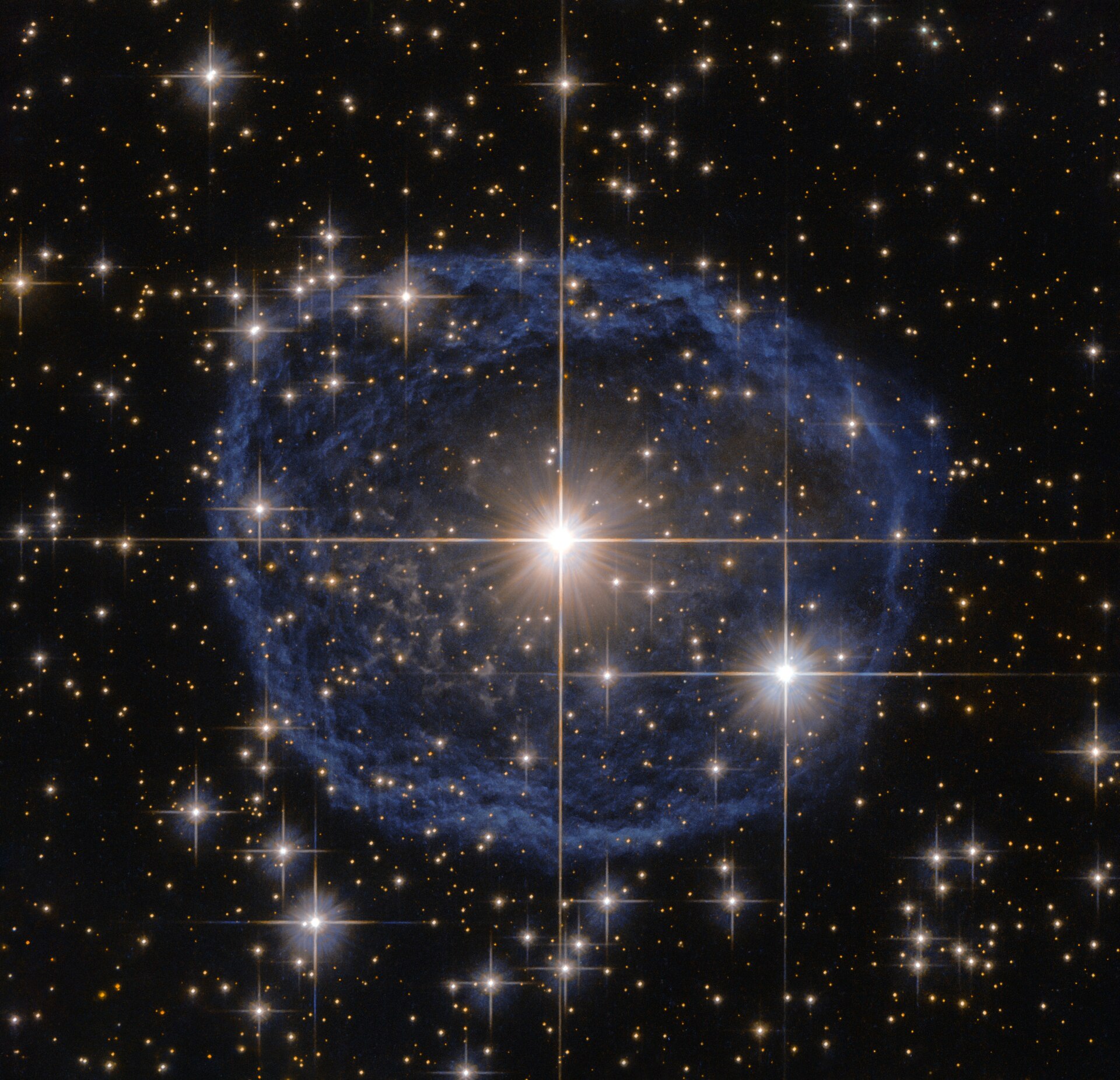
Fig. 100 HST image of Henize 3-519 (field of view is approx 100×100 arcsec). Image credit: ESA/Hubble and NASA. Acknowledgement: Judy Schmidt.

Dynamical ages of young nebulae can be determined from a combination of imaging (apparent size of nebulae) and spectroscopy (expansion velocity of nebulae). By way of example Fig. 100 shows an optical image of the ejecta nebula associated with a hot, luminous evolved star, He 3-519. The physical radius, \(R\), can be obtained if the distance is known. The expansion velocity of a spherical expanding shell, \(v_{\rm exp}\) can be measured from slit or IFU spectroscopy across the nebula, since the projected velocity, \(v(r)\) offset a distance \(r\) from the star will be

\[v(r) = v_{\rm sys} \pm \frac{v_{\rm exp}}{R} (R^2 - r^2)^{1/2}\]

where \(v_{\rm sys}\) is the systemic velocity of the source along our line-of-sight. Examples of fits to receding and approaching halves of the nebula can be seen in Fig. 101. The dynamical age of the nebula, \(\tau_{\rm Dyn} = R/v_{\rm exp}\) follows if \(R\) and \(v_{\rm exp}\) can be obtained. See Example 5.3 for a worked example of He 3-519. Similar approaches are used for young Planetary Nebulae.

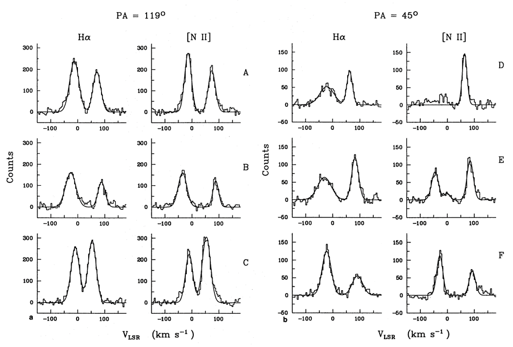
Fig. 101 Gaussian fits to emission lines profiles at different slit locations within the Henize 3-519 nebula, allowing its expansion velocity to be determined (left spectra are at a position angle of 119°, right spectra are for 45° position angle). LSR = Local Standard of Rest, see Fig 1 of Smith, Crowther & Prinja (1994) for further details.

Temperature of a pure hydrogen nebula

The equilibrium gas temperature is determined by the balance between heating and cooling rates. If, on average, energy \(Q\) is injected into the gas in each photoionization, the energy input rate \(\mathcal{G}\) per unit volume is thus

\[\mathcal{G} = \frac{dN_{I}}{dt} Q = \frac{dN_{R}}{dt} Q.\]

On average, at each recombination, energy \(k T_{e}\) is removed from the gas. The reason why this is not \(\frac{3}{2} kT_{e}\) is that the recombination coefficient decreases within increasing electron energy; low energy electrons preferentially recombine. The energy loss rate per unit volume is

\[\mathcal{L} = (k T_{e}) \frac{dN_{R}}{dt}.\]

In equilibrium \(\mathcal{L} = \mathcal{G}\), hence

\[T_{e} = Q/k.\]

\(Q\) depends on the radiation field of the star and also on the distance from the star. If the star radiates as a blackbody at a temperature \(T_{\ast}\) then the average energy injected per photoionization is given approximately by

\[Q \sim k T_{\ast}.\]

We therefore predict that \(T_{e} = T_{\ast}\). For O stars \(3 \times 10^{4}~{\rm K} \leq T_{\ast} \leq 5 \times 10^{4}\) K, so predicted \(T_{e}\) lie in the same range. Observationally nebulae possess significantly lower temperatures (\(\sim 10^{4}\) K), so important coolants have been neglected. For a pure H nebula, there are three additional cooling processes. Thermal plasma emits bremsstrahlung (braking radiation). Electrons can lose energy by collisionally exciting neutral H atoms and also by ionizing them, However, even when these processes are included, gas temperatures of \(\sim 2 \times 10^{4}\) K are predicted, so we must relax our assumption that nebulae are composed only of hydrogen.

Nebulae containing heavy elements

Recalling Fig 96, the spectra of nebulae contain lines emitted by ions of elements other than hydrogen. Indeed, more radiant energy is emitted by other elements than hydrogen. This is somewhat surprising because elements responsible for these lines are much less abundant than hydrogen, and is the case because the process of excitation of these lines is extremely efficient and more than offsets abundance differences.

Forbidden-line cooling

For simplicity, let us focus on oxygen, which turns out to be the most important coolant, and lines its ions radiate are useful for investigating the physical structure of nebulae. Recalling Figure 70, the first ionization potential of oxygen is almost identical to hydrogen. Hence, wherever hydrogen is ionized, we also expect to find ionized oxygen. Unlike hydrogen, however, oxygen van be ionized more than once. The second ionization potential of oxygen has a value χ = 35.1 eV. Although this is much higher than the ionization potential of hydrogen (and singly ionized oxygen), many of the massive stars associated with ionized nebulae emit enough energetic photons to ionize a significant fraction of oxygen to the second state of ionization, This oxygen exists in the forms O⁺ and O²⁺ in H II regions (O³⁺ too exists in PNe too since their central stars are much hotter).

The strongest visual features in PNe and young H II regions lie in the green (4959, 5007Å) and violet (3727, 3729Å). When the first spectroscopy of nebulae were obtained (e.g. William Huggins), these were initially attributed to a mysterious element (unknown on Earth) called nebulium. This is because such lines were not known from laboratory measurements (e.g. Kirchhoff & Bunsen). Ira Bowen noticed that the energy difference between the ground and first excited state of doubly ionized oxygen matched these wavelengths of these lines perfectly (recall Fig. 77). These forbidden lines are not observed in a laboratories since their spontaneous decay rates are so low, τ([O III] 5007Å) \(\sim\) 50s (recalling Figure 58) versus 0.1 millisec for Hβ. They are strongly suppressed at atmospheric densities, owing to collisional de-excitation, but appear in nebulae due to their extremely low densities.

Ions must, of course, be excited into the upper levels from which forbidden emission lines can be emitted. In the case of hydrogen, the mechanism for populating the higher levels is recombination of a free electron with a proton. Recombination plays a negligible role for forbidden lines. Instead collisional excitation is responsible, via the impact of an electron on an ion in the ground state (recall end of Chapter 3). We will consider this cooling process in the low density limit (where collisional de-excitation from the upper levels doesn’t need to be considered). Therefore, the calculate the rate of emission of photons per unit volume by transitions from a particular level, we need to calculate the excitation rate to this level per unit volume.

In the low density limit the timescale that an ion remains in an excited level is much less than the timescale for which an ion remains in the lower level. Therefore we can assume that all ions are present in the lowest energy level. Recalling Eqn (22), the rate of collisional excitation of ion \(I\) from level \(i\) to level \(j\) per unit volume is

\[\dot{N}_{ij} = n_{e} n_{I} C_{ij}(T_{e})\]

where \(C_{ij}\) is provided in Eqn (23). Since each excitation is followed by emission of a photon of energy \(\chi_{ij}\), the rate of loss of energy per unit volume is

\[\mathcal{L}_{ij} = \dot{N}_{ij} \chi_{ij} = n_{e} n_{I} C_{ij}(T_{e}) \chi_{ij}.\]

The number density \(n_{I}\) depends on the proportion of an elements in the form of specific ion. If a fraction \(y_{I}\) of a given element \(z\) is in the form of ion I, then \(n_{I} = y_{I} n_{z}\) where \(n_{z}\) is the number density of nuclei of element \(z\). Further, we need to take account the abundance of element \(z\) relative to hydrogen \(a_{z} (= n_{z}/n_{\rm H})\). We can now calculate the cooling arising from collisional excitation to the \(^{2} D^{\circ}\) state of [O  II] (recall Eqn. 18) for an adopted \(a_{z} = 6 \times 10^{-4}\) as

(35)\[\mathcal{L}_{O+} \sim 1.1 \times 10^{-34} y_{O+} \frac{n_{e} n_{\rm H} }{T_{e}^{1/2}} \exp (-3.89 \times 10^{4}/T_{e}) \]

in units of erg per cubmic cm per second. Now let us estimate the temperature of the gas if we include forbidden line cooling due to O⁺. If all the oxygen present is singly ionized, the equation of energy balance \(\mathcal{L}_{O+} = \mathcal{G}\). Since

\[\mathcal{G} = \frac{dN_{R}}{dt} Q = n^2 \alpha_{B}(T_{e}) kT_{\ast}\]

We find that the equilibrium temperature is given by

\[T_{e}^{1/4} \exp (-3.89 \times 10^{4}/T_{e}) = 2.5 \times 10^{-6} T_{\ast}.\]

Adopting \(T_{\ast} = 4 \times 10^{4}\) K, the calculated equilibrium temperature is \(T_{e} = 8,500\) K. This temperature is in good agreement with observed temperatures, so we have established that forbidden line cooling dominates over other mechanisms. In practice several collisionally excited lines are responsible for cooling H  II regions, including [O  III] λ5007, 51.8μm.

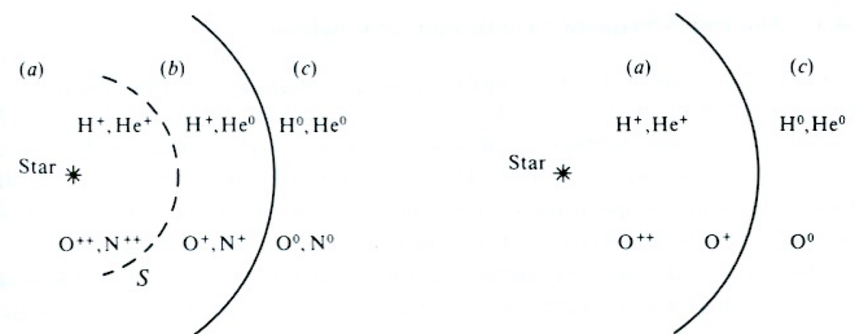
Fig. 102 Ionization stratificaion in a nebula for (left) low temperature ionizing star (\(T_{\ast} < 40\) kK) and (right) high temperature ionizing star (\(T_{\ast} \geq 40\)kK). Fig 5.3 from Dyson & Williams’s Physics of the ISM textbook.

Stratification in nebulae

Oxygen can be present as either singly or doubly ionized in H II regions. Cooling rates depends on the proportion of the element present in that stage of ionization. Narrow-band imaging with filters that isolate e.g. [O II] \(\lambda\lambda\)3727,3729 or [O III] \(\lambda\lambda\)4959,5007 reveal that O²⁺ is more centrally concentrated than O⁺, the latter extending further from the star. This is known as ionization stratification and is illustrated in Fig. 102. For a lower temperature ionizing star (\(T_{\ast} < 40\)kk) helium will be neutral in the outer regions (photons with \(h\nu > 24.6\) eV are required to ionize neutral He), but singly ionized in the central region, together with O²⁺. For a higher temperature ionizing star (\(T_{\ast} \geq\)40k) helium will be mostly ionized throughout the nebula.

Dust extinction

We have previously introduced the dramatic effect that dust extinction has on transmitted spectra (e.g. Fig. 86). Although nebulae lack a continuum, one would be able to determine the interstellar reddening if pairs of lines with known intrinsic ratios are available, following Eqn (31). In reality all emission lines depend on physical conditions, but some depend only slightly on these properties. Case B (optically thin nebula except for Lyman photons) recombination theory reveals that ratios of hydrogen lines are relatively insensitive to \(n_{e}, T_{e}\). By way of example, the intensity ratio of Hα to Hβ is shown in Table 7 for a range of physical conditions. Consequently,

(36)\[\frac{F_{H\alpha}}{F_{H\beta}} = \frac{I_{H\alpha}}{I_{H\beta}} 10^{-c (x_{H\alpha} - x_{H\beta})} = \frac{I_{H\alpha}}{I_{H\beta}} 10^{0.346 c_{H\beta}}\]

using CCM extinction coefficients from Table 6. Adopting \(T_{e} = 1 \times 10^{4}\)K and \(n_{e} = 10^{2}\) cm^-3, \(I(H\alpha)/I(H\beta)\) = 2.86, observed flux ratios permit \(c_{H\beta}\) to be determined, via

(37)\[c_{H\beta} = 2.89 \log \frac{F_{H\alpha}}{F_{H\beta}} -1.32,\]

which can be converted to broad-band dust extinctions via

(38)\[E_{B-V} \sim 0.80 c_{H\beta}.\]

Table 7 Predicted ratios of \(I(H\alpha)/I(H\beta)\) from Case B recombination theory (Hummer & Storey 1987) for various \(T_{e}\) (K) and \(n_{e}\) (cm^-3).

\(T_{e}\)	\(n_{e} = 10^{2}\)	\(n_{e} = 10^{4}\)	\(n_{e} = 10^{6}\)
5,000	3.04	3.00	2.92
10,000	2.86	2.85	2.81
15,000	2.79	2.78	2.75
20,000	2.75	2.74	2.72

Temperature diagnostics

Nebular emission lines are thermally broadened, \(\propto (T_{e}/m)^{1/2}\), so in principle if lines can be spectrally resolved, it is possible to measure electron temperatures. In practice, the gas may be in turbulent motion, so \(\Delta \lambda\), the full-width at half-maximum (FWHM) of a nebular line, at a wavelength λ can be expressed as

\[\frac{\Delta \lambda}{\lambda} = \frac{2}{c} \ln 2^{1/2} \left(\frac{2 k T_{e}}{m} + v_{\rm turb}^2\right)^{1/2}\]

where \(v_{\rm turb}\) is due to the bulk motion of the gas. Lines of different ions need to be observed to identify turbulent velocities and and in practice many nebulae are too faint to observe at high spectral resolution.

Collisional excitation rates are sensitive to electron temperature and excitation energy χ (Eqn (23)) so temperatures can alternatively be determined if any ion exist which possess energy-level structures that result in emission lines from two different upper levels with considerably different excitation energies in the observable wavelength region. In general, ions with ground-state configurations \(s^2 p^2\) are temperature sensitive, including N⁺, O²⁺, S²⁺. Fig 77 reveals that [O III] (and [N II]) are the best examples in the visual. [O III] \(\lambda\lambda\)4959, 5007 occur from the intermediate ¹D level, whereas [O III] λ4363 originates from the upper ¹S level. It is clear that the relative rates of excitation to the ¹S and ¹D levels depend very strongly on \(T_{e}\) so the relative strengths of these lines may be used to measure electron temperatures.

Every excitation of ¹S is followed by emission of a photon at either λ4363 or λ2321, with the relative probabilities given by their relative transition probabilities, i.e. the probability of a λ4363 radiative transition is \(A_{4363}/(A_{4363} + A_{2321})\). Each emission of a λ4363 photon further results in the population of ¹D, which is followed by emission of a λ4959 or λ5007 photon, but this contribution is small in comparison with the direct excitation of ¹D and can be neglected.

At the low density limit, the λ4363 to \(\lambda\lambda\)4959,5007 ratio depends only on atomic physics and the gas temperature \(T_{e}\). The low density limit applies when the density is below the critical density for both ¹D\(_{2}~(6\times 10^{5}\) cm^-3 at K) and ¹S\(_{0}~(3 \times 10^{7}\) cm^-3 at K). Inserting numerical values of the collision strengths and transition probabilities,

\[\frac{I_{4959} + I_{5007}}{I_{4363}} = \frac{7.9 \exp (3.29 \times 10^{4}/T_{e})}{1 + 4.5 \times 10^{-4} n_{e}/T_{e}^{1/2}}.\]

Neglecting the weak \(n_{e}\) dependence, the temperature can be approximated by

\[T_{e} = \frac{3.29 \times 10^{4}}{(\ln I_{5007}/I_{4363} - 1.779)}\]

since \(I_{5007} = 3 \times I_{4959}\) from Chapter 3. The sensitivity of [O III], [N II] and other diagnostic pairs to temperature is shown in Fig. 103. Electron temperatures are typically in the range \(T_{e}\) = 7,000-15,000 K. The [O III] line intensity ratio (λ4959+λ5007)/λ4363 is quite large and is therefore often difficult to measure accurately. Although \(\lambda\lambda\)4959, 5007 are strong lines in many gaseous nebulae, λ4363 is relatively weak, especially at low temperatures (metal-rich regions).

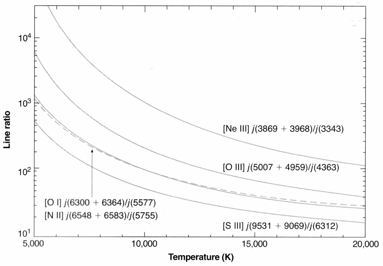
Fig. 103 Calculated variation of forbidden line ratios as a function of \(T_{e}\) in the low density limit (\(n_{e}\) = 1 cm^-3), including [O IIi], [N II]. Figure 5.1 from Osterbrock & Ferland’s AGN².

Density diagnostics

The average electron density in a nebula can be measured by observing the effects of collisional de-excitation. This can be done by comparing the intensities of two lines of the same ion, emitted by different levels with nearly the same excitation energy (so insensitive to temperature) in order that the the relative excitation rates depend solely on collision strengths. If the two levels have different radiative transition probabilities, the relative populations of the two levels will depend on the density, so the ratio of their line intensities will also depend on density.

Ions with ground state conflgurations of \(s^{2} p^{3}\) are density sensitive, including O⁺, Ne³⁺, S⁺, Ar³⁺. The best examples of lines that may be used to measure \(n_{e}\) in the optical are [O II] λ3729/3726 or [S II] λ6717/6731 (recall energy level diagram Fig. 78). Although the oxygen doublet is usually much stronger, the line separations are small so high resolution spectroscopy is required, and these lines lie in the violet part of the spectrum which is preferentially affected by dust extinction. Therefore in practice the [S II] doublet is more commonly used (wider separation, red wavelength).

Let us consider the [O II] doublet in the low density limit, i.e. every collisional excitation is followed by emission of a photon. Since the relative excitation rates of the ²D\(^{\circ}_{5/2}\) and ²D\(^{\circ}_{3/2}\) levels are proportional to their collision strengths, which divide according to their statistical weights, so the ratio of strengths of the two lines is

\[\lim_{n_{e} \rightarrow 0} \frac{I_{3729}}{I_{3726}} = \frac{\Upsilon (^{2}{\rm D}^{\circ}_{5/2} - ^{4}{\rm S}^{\circ}_{3/2})}{\Upsilon (^{2}{\rm D}^{\circ}_{3/2} - ^{4}{\rm S}^{\circ}_{3/2})} = \frac{g(^{2} {\rm D}^{\circ}_{5/2})}{g(^{2} {\rm D}^{\circ}_{3/2})} = 1.5\]

In contrast, at the high density limit, collisional excitations and de-excitations dominate and setup a Boltzmann population ratio. so the relative strengths are in the ratio

\[\lim_{n_{e} \rightarrow \infty} \frac{ I_{3729} }{ I_{3726} } = \frac{g(^{2} D^{\circ}_{5/2})}{g(^{2} D^{\circ}_{3/2})} \frac{A_{3729}}{A_{3726}} = \frac{3}{2} \frac{3.6 \times 10^{-5}}{1.6 \times 10^{-4}} = 0.34.\]

The transition between the high- and low density limits occurs in the neighbourhood of the critical densities which are \(n_{c} = 3 \times 10^{3}\) cm^-3 for \(^{2} D^{\circ}_{5/2}\) and \(n_{c} = 1.6 \times 10^{4}\) cm^-3 for \(^{2} D^{\circ}_{3/2}\). We have previously introduced critical density for the two level atom (end of Chapter 3). More generally it is defined as

\[n_{c}(i) = \frac{\Sigma_{j<i} A_{ij} }{ \Sigma_{j \neq i} C_{ij} }\]

so for \(n_{e} < n_{c}(i)\) radiative de-excitation dominates over collisional de-excitation, while for \(n_{e} > n_{c}(i)\), the reverse is true. Consequently specific lines are sensitive to electron density in the vicinity of their critical densities, as shown in Fig. 104 for [O II] and [S II]. Both diagnostics are sensitive to relatively low density nebulae (typical of H II regions and PNe), with other diagnostics necessary for denser environments.

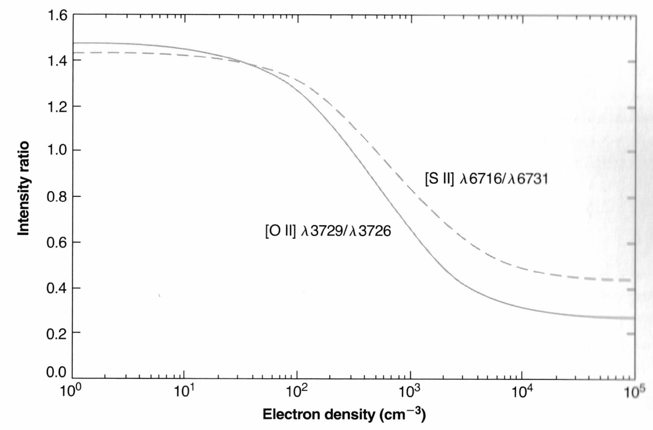
Fig. 104 Calculated variation of [O II] (solid) and [S II] (dashed) intensity ratios as functions of \(n_{e}\) at \(T_{e}\) = 10,000 K. At other temperatures the plotted curves are very nearly correct if the horizontal scale is taken to be \(n_{e} (10^{4}/T_{e})^{1/2}\). Figure 5.8 from Osterbrock & Ferland’s AGN².

For example, low lying energy levels of C III involve the ground state \(^{1}S_{0}\) and first excited term \(^{3}P^{\circ}\) which is split into three levels \(^{3}P_{0}^{\circ}\), \(^{3}P_{1}^{\circ}\) and \(^{3} P_{2}^{\circ}\) (recall Fig. 75). The \(^{3}P_{1}^{\circ}\) to \(^{1}S_{0}\) transition at 1909Å is semi-forbidden (electric dipole selection rules are followed apart from \(\Delta S = 0\)) so has an Einstein \(A\) value of 114 s^-1. The \(^{3}P_{2}^{\circ}\) to \(^{1}S_{0}\) transition at 1907Å is forbidden by electric dipole and magnetic dipole rules since \(\Delta J = 2\) so has a very small Einstein \(A\) value of 0.005 s^-1. The huge difference in their lifetimes is reflected in their critical densities so the relative strength of C III] 1909Å to [C III] 1907Å can be used as a diagnostic for higher density regions than [S II] although their location in the UV and small wavelength separation (requiring high resolution) restricts their use to bright nebulae (e.g. Feibelman et al. 1981). [O II] and C III] are detected in the high-redshift galaxy GN-z11, but their components are blended , with [S II] redshifted out of the JWST-NIRSpec wavelength range (Fig 4).

Ionizing fluxes

With the exception of very nearby B stars lying along low density sight-lines (Fig. 89), the Lyman continuum (≤ 912Å) from hot stars cannot be directly observed since EUV photons are absorbed by neutral hydrogen along the sight-line. Observations of gaseous nebulae may be used to indirectly find the number of ionizing photons emitted. If the nebula around the star is optically thick in the Lyman continuum, it will absorb all the ionizing photons emitted. Therefore the number of ionizations per unit time will equal the number of ionizing photons emitted per unit time, and in equilibrium is balanced by the number of recaptures per unit time, i.e.

\[\int_{\nu_0}^{\infty} \frac{L_{\nu}} {h \nu} d\nu = Q_{0} = \int_{0}^{r_{1}} n_p n_{e} \alpha_{B}(H^{0}) dV,\]

where \(L_{\nu}\) is the luminosity of the star per unit frequency interval, and \(\alpha_{B}\) is the case B recombination coefficient for hydrogen.

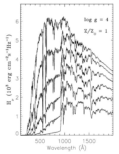
Fig. 105 Predicted fluxes for dwarf O stars at solar metallicity for temperatures of 55kK, 50kK, 45kK, 40K, 35kK and 30kK (top to bottom) from Lanz & Hubeny (2003). The number of Lyman continuum photons, \(Q_{0}\) (≤ 912Å) is very sensitive to stellar temperature, as is the number of helium continuum photons, \(Q_{1}\) (≤ 504Å). O stars are negligible sources of He⁺ ionizing photons (\(Q_{2} \leq 228\)Å).

The luminosity of the entire nebula in a particular emission line, say Hα, also depends on recombinations throughout its volume,

(39)\[L(H\alpha) =h \nu_{H\alpha} \int_{0}^{r_{1}} n_p n_e \alpha_{H\alpha}^{eff} dV,\]

so

\[Q_{0} = \frac{\alpha_{B}(H^{0})}{\alpha_{H\alpha}^{\rm eff}} \frac{L(H\alpha)}{h \nu_{H\alpha}}.\]

i.e. the total number of ionizing photons can be determined from \(L(H\alpha)\) if the ratio \(\alpha_{B}(H^{0})/\alpha_{H\alpha}^{\rm eff}\) is known. The former is given in Eqn (33) while that for Hα is

(40)\[% 2.87 * 3.03e-14 at 10^4K according to Table 4.2 of AGN^2 \alpha_{H\alpha}^{\rm eff} = 8.6 \times 10^{-14} \]

in units of cubic cm per second at \(T_{e} = 10^{4}\) K and \(n_{e} = 10^{2}\) cm^-3 according to Table 4.4 of Osterbrock & Ferland (the ratio depends only weakly on \(T_{e}\), Pequignot et al. 1991). Any other recombination line could be used instead of Hα. The expression for \(Q_{0}\) given above assumes that all Lyman continuum photons are absorbed by the nebula, so it is described as ‘ionization bounded’. If some ionizing photons were to leak out this method would underestimate the true total, and the nebula is described as ‘density bounded’. Inserting recombination coefficients for \(T_{e} = 10^{4}\) K and \(n_{e} = 10^{2}\) cm^-3,

\[Q_{0} = 7.4 \times 10^{11} L(H\alpha)\]

for \(L\)(Hα) in erg s^-1, requiring knowledge of the distance to the nebula (\(L\)(H\(\alpha) = 4 \pi d^2 I(H\alpha)\)) and dust extinction (Eqn. (36)).

Table 8 Physical properties of OB stars in the cluster responsible for the Orion Nebula. Properties from Simon-Diaz et al. (2005) and Draine’s ISM textbook for \(\theta^{1}\) Ori B, except that ionizing photons are obtained from Lanz & Hubeny (2003).

Star	Spect Type	\(T_{\ast}\) (kK)	\(\log L/L_{\odot}\)	\(Q_{0}\) (s-1)
\(\theta^{1}\) Ori A	B0.5 V	30	4.45	\(2.5\times 10^{47}\)
\(\theta^{1}\) Ori B	B3 V	18	3.2
\(\theta^{1}\) Ori C	O7 V	39	5.31	\(1.1\times 10^{49}\)
\(\theta^{1}\) Ori D	B0.5 V	32	4.47	\(6.0\times 10^{47}\)

This approach is relatively straightforward for planetary nebulae, since a single hot star is responsible for the ionized nebula. H II regions however usually host many OB stars. By way of example, let us consider the Orion Nebula (Fig. 93). Physical properties of the four brightest OB stars in the ‘Trapezium’ cluster (\(\theta^{1}\) Ori) responsible for the nebula are shown in Table 8. Amongst these, the hottest (and most massive) star dominates the number of ionizing photons emitted. This is because the Lyman continuum production rate is a very steep function of temperature.

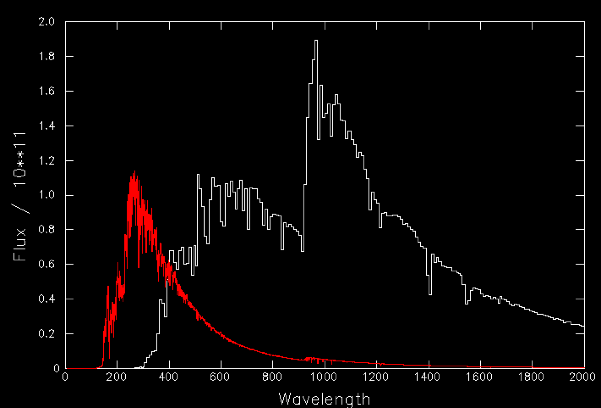
Fig. 106 UV spectral comparison between a massive O star (white) and low-mass CSPN (red), highlighting the overall lower output of a PN central star, albeit significantly hotter (harder UV photons), some of which are at wavelengths below 228Å, and so are capable of doubly ionizing helium.

This is illustrated in Fig 105, such that the most massive stars (which are the hottest on the main sequence) dominate the number of ionizing photons. Only the hottest O stars emit significant numbers of He⁰ ionizing photons \(Q_{1} (\leq\) 504Å), while negligible He⁺ ionizing photons \(Q_{2} (\leq\) 228Å) are produced by O stars. Only a subset of central stars of planetary nebulae (CSPNe) or hot, evolved massive stars (Wolf-Rayet stars) are sources of significant \(Q_{2}\) photon fluxes, capable of producing He II recombination lines (e.g. λ1640, λ4686). Fig. 106 presents a comparison between the high energy UV output of a massive O star and CSPN.

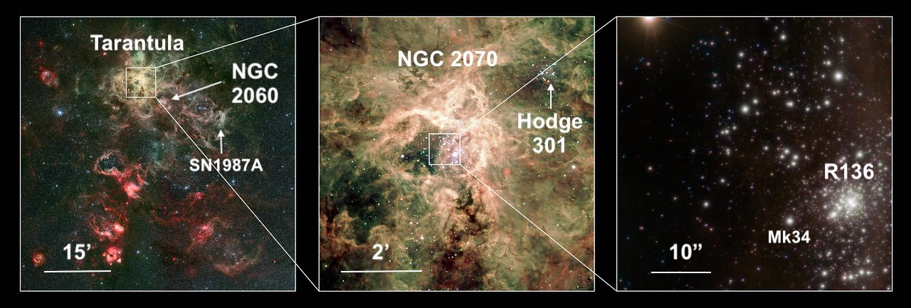
Fig. 107 left Optical colour composite image of the Tarantula Nebula in the LMC with the MPG/ESO 2.2m Wide Field Imager, centre optical VLT/FORS2 image of the central ionizing nebula; right near-infrared VLT/MAD image of the central R136 star cluster. From Crowther (2019).

The Orion nebula is typical of compact H  II regions, but much larger star-forming regions exist in the Milky Way (e.g. Carina Nebula) and beyond. These giant or supergiant H  II regions are host to tens or hundreds of massive stars. For example, the Tarantula Nebula in the LMC has a cumulative ionizing photon output of \(Q_{0} \sim 10^{52}\) s^-1 (Crowther 2019), a thousand times higher than Orion, owing to the presence of hundreds of O stars, including some very massive stars (\(\geq 100 M_{\odot}\)) that emit as much as \(Q_{0} = 5\times 10^{50}\) s^-1. For such rich regions, the OB population is characterized in terms of the equivalent number of ‘representative’ O7 dwarfs,

\[Q_0 = N_{\rm O7V} Q_0^{\rm O7V}\]

for which \(Q_{0}^{\rm O7V} = 10^{49}\) s^-1. Consequently \(N_{\rm O7V}\) = 1 for Orion Nebula, and \(N_{\rm O7V}\) = 1000 for the Tarantula Nebula - see Fig. 107.

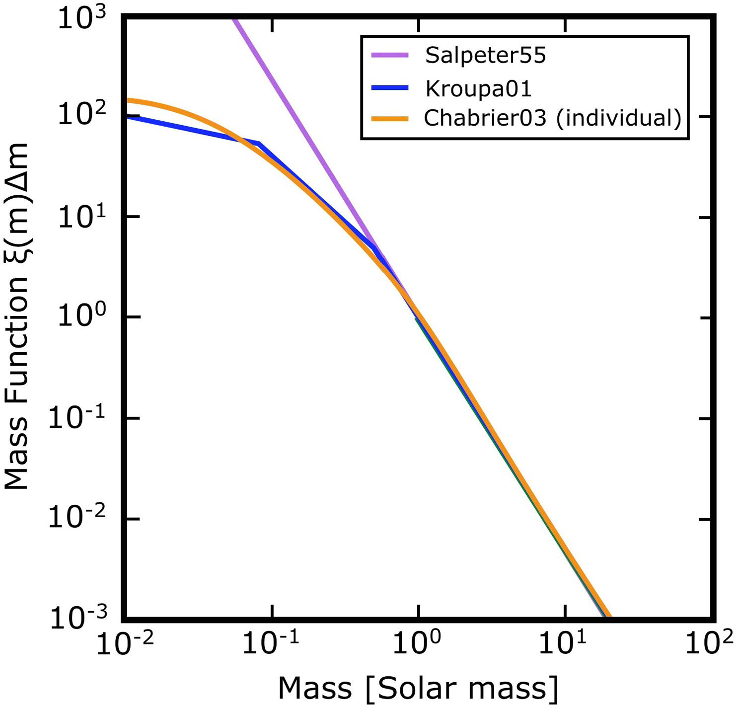
Fig. 108 Stellar Initial Mass Function from Lamers & Levesque Understanding Stellar Evolution textbook showing a steep power law for massive stars (Salpeter-like), and flattening for low mass stars \(\sim 0.1-1.0 M_{\odot}\) (Kroupa or Chabrier-like).

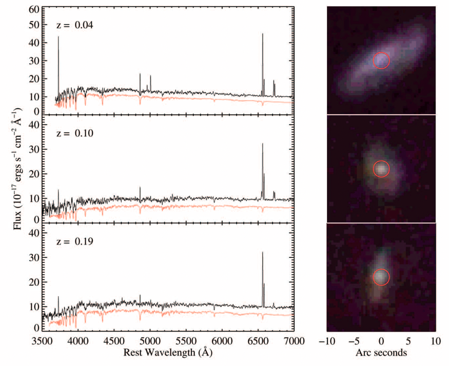
Fig. 109 Representative images (right) and spectra (left) of star-forming galaxies at \(z\) = 0.04, 0.01, 0.19 from SDSS fibre spectroscopy. Red spectra (offset for clarity) represent stellar continuum models allowing nebular emission lines to be identified. Tremonti et al. (2004)

The Hα emission-line luminosity can also be used as an indicator of the current star formation rate of an entire galaxy. For this, one needs to make assumptions about the initial mass function (IMF), since observations (including Orion) reveal that the majority of stars form with masses below the Solar value, such that high mass stars (which dominate ionizing outputs of star-forming regions) are rare, as shown in Fig. 108. For a Salpeter-like IMF, the star-formation rate (in \(M_{\odot}\) yr^-1) can be determined according to Kennicutt (1988) via

\[{\rm SFR} = 7.9 \times 10^{-42} L(H\alpha) = 1.08 \times 10^{-53} Q_{0}\]

with \(L\)(Hα) in erg s^-1. For a more realistic Kroupa- or Chabrier-like IMF, inferred star formation rates need to be adjusted (following Brinchmann et al. 2004) as follows:

\[% factor 1.5 according to Brinchmann et al 2004 {\rm SFR} = 5.2 \times 10^{-42} L(H\alpha) = 7.2 \times 10^{-54} Q_{0}.\]

This approach has been applied to hundreds of nearby galaxies, most recently accounting for star-formation that is visibly obscured due to dust (Kennicutt et al. 2009). By way of example, the star formation rates of the LMC and SMC are 0.2 \(M_{\odot}\) yr^-1 and 0.04 \(M_{\odot}\) yr^-1, respectively. Star-formation rates of thousands of galaxies at \(z>0\) have also been determined, often using SDSS fibre spectroscopy (Fig 109).

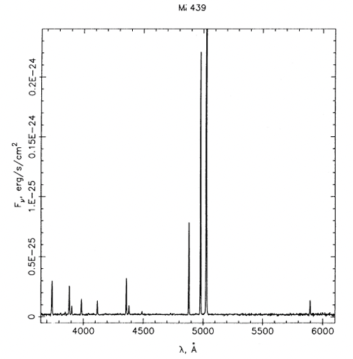
Fig. 110 The optical spectrum of a typical H  II galaxy, Mich 439 from Campbell et al (1986), revealing exceptionally strong [O  III] \(\lambda\lambda\)4959,5007

For comparison, the Milky Way is believed to be forming stars at a rate of \(\sim\)2 \(M_{\odot}\) yr^-1 and some galaxies are actively forming stars at very high rates (10s to 100s of \(M_{\odot}\) yr^-1), known as starburst galaxies. Intensely star-forming H II galaxies include so-called Green Pea galaxies. The optical spectrum of a H II galaxy is shown in Fig. 110. Green peas are so-named since SDSS imaging revealed a compact, green appearance (Fig 111) owing to strong [O III] \(\lambda\lambda\)4959-5007 emission lines redshifted into the SDSS \(r\)-filter at \(z\sim0.2\), green being the colour represented by the \(r\) band in colour composites.

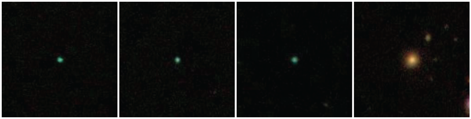
Fig. 111 SDSS \(g, r, i\) (blue, green, red) composite 50×50 arcsec² images of three Green Pea H  II galaxies (left) and an elliptical galaxy (right) at the same redshift of \(z\sim0.2\). Cardamone et al. (2009).

Abundances from HII regions

Optical emission lines observed in ionized nebula are optically thin, bright (detectable in distant star-forming regions) and span a range of elements (e.g. H, He, N, O, Ne). Therefore they have several advantages over stellar atmospheres for abundance studies, which often require high S/N, high spectral resolution observations and the need to incorporate radiative transfer effects (details to follow in PHY305). In general, direct abundance determinations from nebulae can be divided into whether these are collisional or radiative (recombination) in origin. Mass fractions of hydrogen, helium and metals are usually denoted \(X, Y\) and \(Z\).

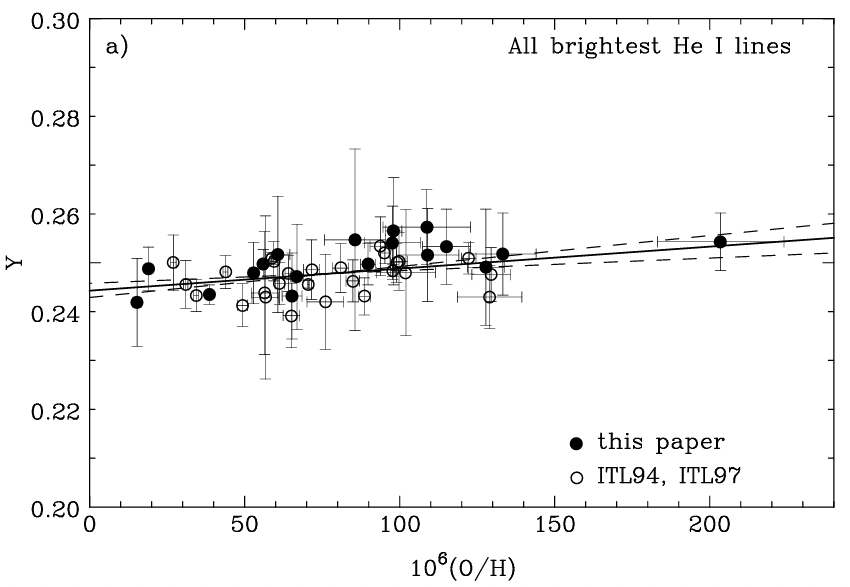
Fig. 112 Helium mass fractions (\(Y\)) of metal poor H  II regions from Izotov et al. (1998).

Recombination lines

The strength of recombination lines scales with the number density of ions responsible for the emission line (protons for hydrogen, He ions for He i lines, He²⁺ for He II lines) as well as electron density and relevant recombination coefficient (recall Eqn (39)). Consequently it is relatively straightforward to determine helium abundances from recombination lines of He I (and He II in PNe) since the number density of helium is only one order of magnitude lower than hydrogen. Helium abundances (by mass, \(Y\)) of metal poor H II regions from neutral He recombination lines are presented in Fig. 112 allowing a determination of the primordial He content.

In contrast, the number densities of other elements are much lower than H (or He) so their recombination lines are extremely weak. Recombination lines have been used to determine abundances of metals in nearby PNe, but this approach is not viable in most distant H II regions. For example, the O II \(3p ^{4}D^{\circ} - 3s ^{4}P\) multiplet is prominent in NGC 7009 (recall Fig. 97). If \(I(\lambda)\) is the intensity of a O II recombination line, then

\[\frac{N(O^{2+})}{N(H)} = \frac{\lambda}{4861} \frac{\alpha_{\rm eff}(H\beta)}{\alpha_{\rm eff}(\lambda)} \frac{I(\lambda)}{I(H\beta)}\]

following Liu et al. (1995), where \(\alpha_{\rm eff}\) represents the effective recombination coefficient, noting that such lines provide abundances of the relevant recombining ion (O²⁺ for O II recombination lines, H⁺ for Hβ). Metal abundances measured from recombination lines should be more robust than those obtained from other methods (see below) since both heavy-element and hydrogen recombination lines have similar temperature dependencies.

Collisionally excited lines

Recalling the optical spectrum of the Orion nebula (Fig. 96) numerous strong collisionally excited lines of N, O, Ne, S, Ar are observed. In contrast to recombination lines, their strengths depend sensitivity on temperature, since recombination coefficients are replaced with collisional excitation coefficients \(C_{ij}(T_{e})\) (Eqn (23)) as well as the fraction of excitations to level \(j\) that are followed by emission of a photon in the line observed. Reliable temperatures must be determined using the approach set out earlier in this Chapter. In general, only lower limits to metal abundances can be determined since nebulae are stratified, so photoionization models are required to provide ionization correction factors (ICFs) for unobserved ionization stages.

Fortunately, oxygen has strong collisional lines of O⁺ (3726, 3729Å) and O²⁺ (4959, 5007Å) at optical wavelengths, which together represent the dominant ionization stages of this element in H II regions (O³⁺ is predicted in PNe). Therefore if it is possible to determine their ionic abundances (relative to hydrogen) the total oxygen abundance in gas phase will be

\[\frac{N(O)}{N(H)} = \frac{N(O^+)}{N(H)} + \frac{N(O^{2+})}{N(H)}\]

In practice, abundances of O⁺ and O²⁺ can be determined from intensities of the blend of λ3726 and 3729 [O II] and λ5007 [O III] with respect to Hβ, together with emissivities ε (sensitive to \(T_{e}\)) as follows

\[\frac{I([OII]~3726+3729)}{I(H\beta)} = \frac{\epsilon([OII]~3726+3729)}{\epsilon(H\beta)} \times \frac{N(O^{+})}{N(H)}\]

\[\frac{I([OIII]~5007)}{I(H\beta)} = \frac{\epsilon([OIII]~5007)}{\epsilon(H\beta)} \times \frac{N(O^{2+})}{N(H)}\]

Emissivities for Hβ involve recombination coefficients and electron densities, whereas those for forbidden lines involve collisional excitation coefficients. Level populations and line emissivities can be determined from numerical codes, which include equib (Howarth & Adams (1981), fivel (De Robertis et al. 1987), nebular (Shaw et al. 1998) and PyNeb (Luridiana et al. 2015).

Most measurements of the abundances of heavy elements in H II regions use a combination of collisionally excited forbidden lines and hydrogen recombination lines. Metallicity gradients of star-forming disk galaxies have been determined using this approach (e.g. Vila-Costas & Edmunds 1992), including our own Milky Way (Deharveng et al. 2000. Physically the gas will be hotter in low-metallicity nebulae, to compensate for fewer coolants. Forbidden lines can only be converted into abundances if the electron temperature is well measured, which requires detection of the faint ‘auroral’ [O III] λ4363 line. This line is very faint in low temperature nebulae (Fig. 103) so, peculiarly, metal abundances are harder to measure in metal-rich nebulae. This is exascerbated by contamination from [Fe II] λ4360 in intermediate resolution observations (Curti et al. 2017).

Table 9 compares elemental abundances obtained from spectroscopic analysis of the Sun (Magg et al. 2022) and the Orion Nebula (Esteban et al. 2004), presented on the (unusual) astronomical scale

\[A(i) = \log \frac{N(i)}{N_{\rm H}} + 12.\]

Most nebular-derived elemental abundances are from collisional lines (including ICFs where necessary) with the exception of helium and carbon (lacking optical collisional lines). Differences between gas phase nebular abundances and solar abundances arise from depletion onto dust grains (\(\sim\)0.1 dex for C and O, more significant for Fe). Once these are incorporated, differences between nebular abundances in the Orion Nebula and Solar photosphere are modest, indicating that there has been relatively little chemical enrichment in the gas phase abundances of the Milky Way thin disk in the last 5 Gyr. For example, contemporary oxygen abundances in the Solar photosphere are \(\log N(O)/N(H)+12 = 8.77\) versus 8.73 for the Orion Nebula.

Table 9 also provides abundances by mass (in percent) suggesting \(Z_{\odot} \sim 0.017\), dominated by O, C, Ne, Fe and N. The carbon abundance is particularly challenging to determine from nebulae since most of the nebular lines are observed in the UV (C IV λ1548-1551, C III] 1909) with only very weak recombination lines detected in the visual (e.g. C II λ4267, C III λ4647-4651). Iron is usually adopted as the primary tracer of ‘metallicity’ from stellar studies, whereas oxygen is used as a ‘metallicity’ proxy from nebular studies (iron lines are weak and depleted on dust grains). Consequently, a concise notation for metallicities with respect to the Sun (Orion) are often used, e.g.

\[[O/H] = \left(\log \frac{N(O)}{N_{\rm H}}\right)_{HII} - \left(\log \frac{N(O)}{N_{\rm H}}\right)_{\odot}\]

For example, [O/H] = -0.4 dex for HII regions in the LMC, and \(-\)0.7 dex in the SMC.

Table 9 Elemental abundances by number, \(A(i)\), in the Solar photosphere (Magg et al. 2022) and Orion Nebula (Esteban et al. 2004). Nebular results from recombination lines (R) are indicated. The final column provides mass fractions, \(X_{i}\)

Element	Solar	Orion Nebula	Mass
H	12	12	74%
He		10.99 (R)	24%
C	8.56	8.42 (R)	0.32%
N	7.98	7.73	0.10%
O	8.77	8.67	0.70%
Ne	8.15	8.05	0.21%
Mg	7.55		0.06%
Si	7.59		0.08%
S	7.16	7.22	0.03%
Fe	7.50	6.23	0.13%

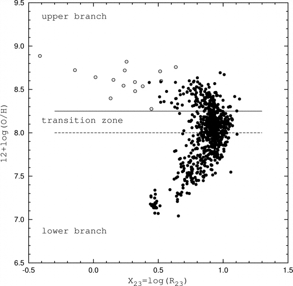
Fig. 113 Oxygen abundances versus \(\log R_{23}\) for extragalactic H II regions from Pilyugin & Thuan (2005). Horizontal lines show the boundaries between the lower and upper branches.

Strong lined calibrations

As noted above, reliable temperatures are required in order to determine metal abundances from collisional lines, yet critical diagnostics such as λ4363 [O III] and λ5755 [N II] are exceptionally weak, especially at low nebular temperatures (metal-rich nebulae). Consequently, a number of calibrations have been developed which rely solely on strong nebular lines, informed by either abundances from direct \(T_{e}\) determinations or theoretical predictions from photoionization models.

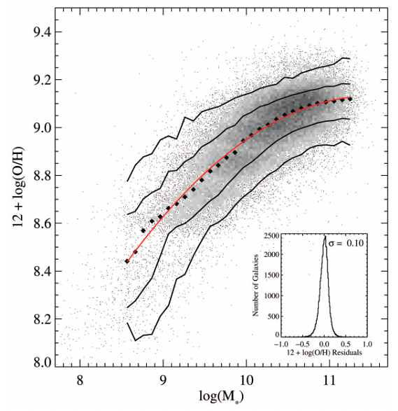
Fig. 114 Mass-metallicity relation for 53,000 SDSS emission-line galaxies obtained from \(\log R_{23}\) (Tremonti et al 2004).

\(R_{23}\)

Historically, the most widely used strong-line calibration involved the ratio of the strong [O II] and [O III] collisional lines with respect to Hβ, first introduced by Pagel et al. (1979). This ratio is known as \(R_{23}\) and is defined as follows:

\[R_{23} = \frac{I([OII] 3726+3729) + I([OIII] 4959+5007)} {I(H\beta)}\]

Figure 113 compares \(\log R_{23}\) with direct measurements of oxygen abundances (from \(T_{e}\)) for large numbers of extragalactic H II regions. It is apparent that high \(R_{23}\) ratios suggest metal poor H II regions (recall \(\log N(O)/N(H)+12 = 8.75\) for the Sun) whereas low \(R_{23}\) ratios are double valued, either very metal poor for the lower branch, or metal-rich (solar-like) for the upper branch. Consequently, this diagnostic is often inconclusive when used in isolation. Nevertheless, it has been applied to thousands of low redshift emission line galaxies observed with SDSS, revealing a clear mass-metallicity relation (Fig. 114).

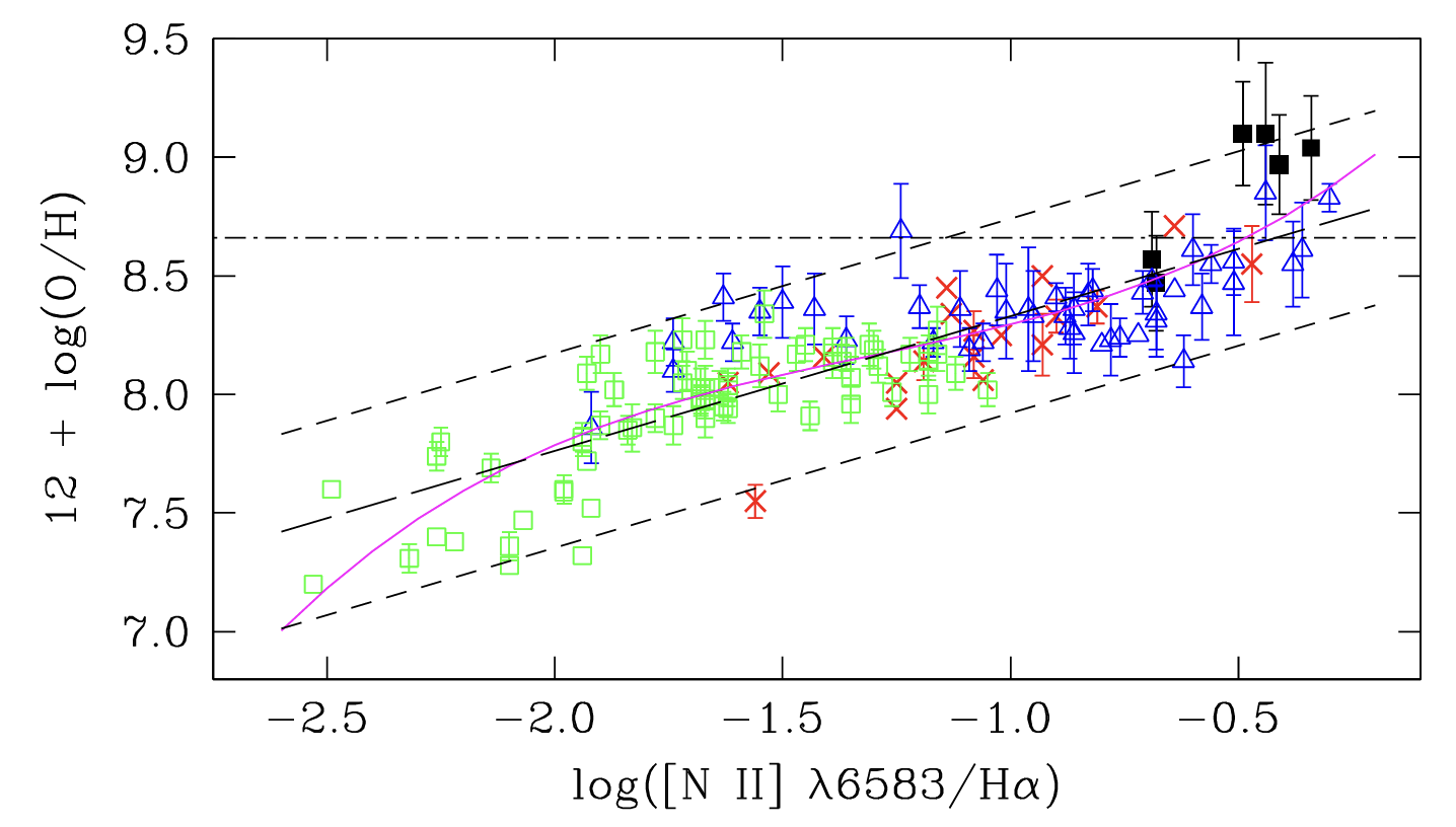
Fig. 115 Oxygen abundance versus N2 for extragalactic H II regions from Pettini & Pagel (2004). The horizontal dot-dash line shows the solar abundance.

N2

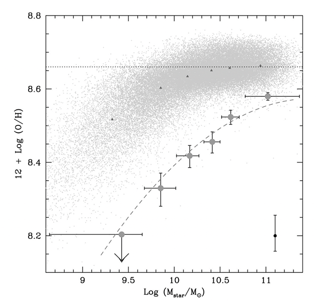
Fig. 116 Stellar mass metallicity relation plot for low redshift SDSS galaxies (small symbols) plus \(z\sim2.3\) galaxies

An alternative strong-line calibration involves the ratio of [N  II] λ6584 to Hα, known as N2,

\[N2 = \log \left(\frac{I([NII]~6584)}{I(H\alpha)} \right).\]

Although [N II] λ6584 is much weaker than [O III] λ5007 (these are isoelectronic transitions, recall Fig. 77), it has the advantage that it lies adjacent to Hα so their ratio is insensitive to dust extinction. Various N2 calibrations exist in the literature, with a least squares fit

(41)\[12 + \log(O/H) = 8.90 + 0.57 \times N2\]

from Pettini & Pagel (2004) most widely used, as shown in Fig. 115. In contrast to the \(R_{23}\) diagnostic, there is a monotonic relation between the N2-index and oxygen content for sub-solar metallicities, although there remains a sizeable dispersion in O/H for a given N2-index (± 0.41 dex). This index has been widely used for high redshift galaxies, since these lines are redshifted to the near-IR (K-band) at \(z\sim2.5\) and can be studied to higher redshift with JWST. Fig 116 shows increasing [N II] strengths with stellar mass for \(z\sim\)2.3 galaxies (albeit lower than \(z\)=0.1 galaxies of the same mass from SDSS).

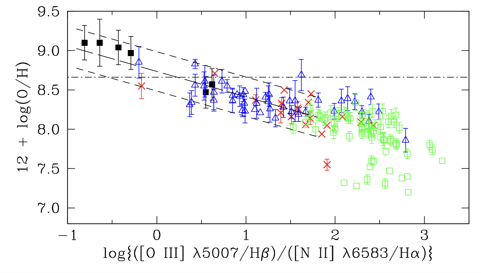
Fig. 117 Oxygen abundance versus O3N2 for extragalactic H  II regions from Pettini & Pagel (2004). The horizontal dot-dash line shows the solar abundance.

O3N2

The final strong-line calibration that we shall consider involves two pairs of line ratios, [O  III] λ5007 to Hβ (O3), and [N  II] λ6584 to Hα (N2), i.e. O3N2, first introduced by Alloin et al. (1979)

\[O3N2 = \log \left( \frac{I([OIII]~5007/H\beta)}{I([NII]~6584/H\alpha)} \right)\]

Fig. 117 shows how this index varies with oxygen abundance, with a tight relationship except at high O3N2 values. Pettini & Pagel (2004) provide a least-squares linear fit to data in the range \(-1 < O3N2 < +1.9\),

(42)\[12 + \log(O/H) = 8.73 - 0.32 \times O3N2\]

with 95% of the measurements within 0.25 dex. Other diagnostics are available, including predictions from photoionization models (Kewley & Dopita 2002) and updated empirical calibrations of N2 and O3N2 (e.g. Curti et al. 2017, their Fig 9).

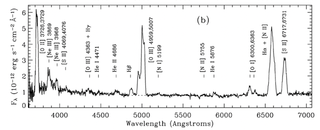
Fig. 118 Integrated optical spectrum of the Crab SNR from Smith (2003). [S II] and [O I] lines are unusually strong with respect to H II regions. Emission lines are broad due to the high temperature of SNR.

Shock-heated versus photoionized regions

So far we have focused on nebulae photoionized by stars (OB-type or central stars of PNe). Recalling Fig. 92, nebulae can also be shock-ionized (e.g. supernova remnants). SNR exhibit emission lines, many in common with H II regions (H, He, [O II-III], [N II], [S II] etc. Indeed for the Crab nebula, standard nebular diagnostics [S II] and [O III] infer \(n_{e} \sim 10^{3}\) cm^-3 and \(T_{e} = 15,000\) K. In contrast with H II regions, SNR show a broader range of ionization stages, ranging from [O I] to He II as shown in Fig. 118. Gas is instantaneously heated by the ionization front from the supernova blast wave, and cools by radiation. Recombination lags behind cooling so a long, partially ionized region is created (producing strong collisionally excited lines of [O I] and [S II].

Consequently it is possible to separate SNR from H II regions using suitable diagnostic diagrams (involving [O I]/Hα or [S II]/Hα). Hα to Hβ ratios also exceed Case B recombination, owing to collisional excitation of Hα from its ground level in a process linked to X-rays (discussed in Section 11.5 of Osterbrock & Ferland’s AGN² textbook).

Photoionization by stars versus active galactic nuclei

There are a small fraction of galaxies with ionized gas that are not associatd with OB stars. Examples include Seyfert galaxies, radio galaxies and quasars. These are collectively known as AGN. Most techniques developed for H II regions and SNR are also applicable to AGN. Spectroscopically, Seyfert 1 galaxies exhibit very broad H and He lines, plus narrower forbidden lines, while Seyfert 2 galaxies show similar widths for permitted and forbidden emission lines. Narrow emission lines are analogous to H II regions, except that the. range of ionization is considerably greater in AGN ([O I], [Ne V], [Fe VII]), indicating a much harder photoionizing source than OB stars. One can distinguish between H II regions and AGN using various emission line intensity ratios. These diagnostic diagrams are collectively known as BPT diagrams after Baldwin, Phillips & Terlevich (1981). Fig. 119 shows the location of SDSS emission line galaxies which are photoionized by stars (H II galaxies) or active galactic nuclei (AGN), separated by the red line in each case.

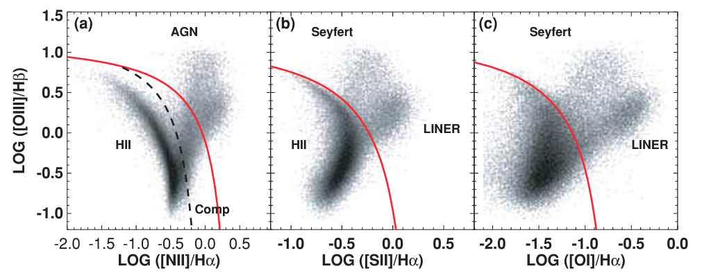
Fig. 119 BPT diagrams for H II regions versus active galaxies (AGN, Seyfert and LINERs) from Kewley et al. (2006). The division between star-forming galaxies and AGN is shown by the red line (Kauffmann et al. 2003).

JWST spectroscopy

High redshift galaxies

One of the primary goals of JWST is the (photometric) identification and (spectroscopic) characterisation of very high redshift galaxies. Prior to JWST, detection of galaxies at redshifts above \(z\sim 5\) was challenging since UV light from galaxies shifts into the red/infrared part of the spectrum. Ground-based observations are affected by strong airglow emission (recall Fig. 48) while the design of HST was originally focused on UV/optical observations.

Table 10 Observed wavelengths of the Lyman break (912 Ang) and Lyman α (1216 Ang) for high-z galaxies, including the rest frame for light associated with JWST’s F444W filter

\(z\)	Age (Myr)	Lyman break	Lyman α	JWST/F444W
4	1550	4650Å	6080Å	Sloan \(z\)
8	640	8208Å	1.09 μ m	Sloan \(g\)
12	370	1.19 μ m	1.58 μ m	Sloan \(u\)
16	250	2.55 μ m	2.07 μ m	NUV

High redshift galaxies are usually detected by a UV dropout (Lyman break) technique. A video showing this technique can be found at

{https://​www​.youtube​.com​/watch​?v​=​6dR96S0HfJo

At low redshift, galaxies become invisible below the Lyman break ({math}`\lambda_0 = 912 Ang) since ionizing EUV photons are absorbed by the intergalactic medium. At very high redshift, the Lyman α forest suppresses stellar emission below Ly α (recall Fig. 7) as illustrated via

https://​www​.youtube​.com​/watch​?v​=​6Bn7Ka0Tjjw

Table 10 shows the observed wavelengths that Lyman α is redshifted to for various high redshift sources, including ages (obtained from Ned Wright’s Cosmic Calculator adopting \(H_{0}\) = 70 km s^-1 Mpc^-1, \(\Omega_{M}\) = 0.286 and a flat universe (\(\Omega_{vac} = 1 - \Omega_{M}\)) Consequently Lyman α is redshifted to 1.58μm for a galaxy at \(z=12\) so this would be expected to dropout in filters below this wavelength (e.g. JWST’s F150W) but appear in longer wavelength filters (e.g. JWST’s F200W). Light associated with JWST’s F444W filter would correspond to rest frame ultraviolet filter (\(\sim 3400\) Angstrom, corresponding to Sloan \(u\)).

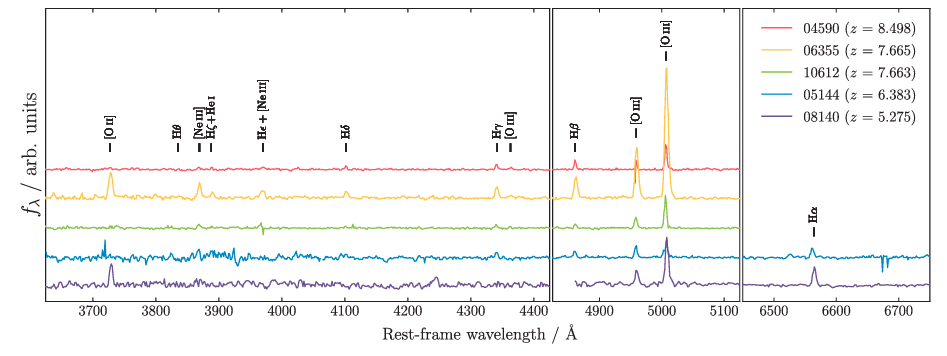
Fig. 120 JWST NIRSpec spectroscopy of \(5 < z < 9\) emission line galaxies from early release observations of the SMACS J0723.3-743 galaxy cluster (Carnall et al. 2023).

By way of example, the first JWST deep field imaging with NIRCam involved the \(z=0.39\) SMACS J0723.3-743 galaxy cluster. Associated NIRSpec spectroscopy revealed a number of high redshift gravitationally lensed galaxies, displaying permitted (H) and forbidden ([O II-III]) emission lines, allowing precise spectroscopic redshifts. Examples from Carnall et al. (2023) are presented in Fig. 120. The presence of [O III] λ4363 and λ5007 permits a direct temperature determination of these galaxies, from which oxygen abundances can be determined (avoiding the uncertainties of strong-line calibrations). The mass-metallicity relation of these galaxies is compared to low redshift galaxies (from CLASSY survey) in Fig. 121.

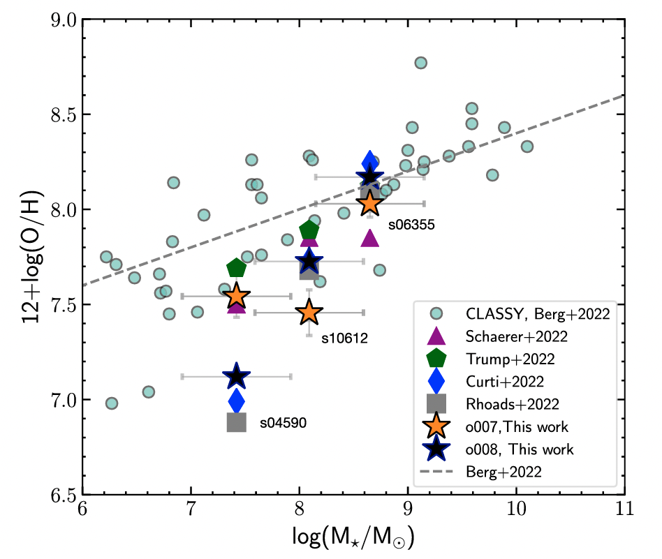
Fig. 121 Mass-metallicity relation for \(z>7\) galaxies from the SMACS J0723.3-743 field, obtained from \(T_{e}\) determinations, together with low redshift galaxies from the CLASSY survey. Reference: Arellano-Cordova et al. (2022)

Even higher redshift (\(10 < z < 13\)) galaxies have subsequently been detected from NIRCam photometric surveys of larger regions and follow-up NIRSpec spectroscopy (e.g. JADES, Robertson et al. 2023) as shown in Figures 122-123. Shallow spectroscopy of these sources achieves low S/N (they are not gravitationally lensed) but high quality spectroscopy is attained for UV luminous high-redshift galaxies such as GN-z11 shown in Fig. 4 which shows emission lines from [O II] λ3727, [O III] λ4363, CIII] λ1909 and NIV] λ1486.

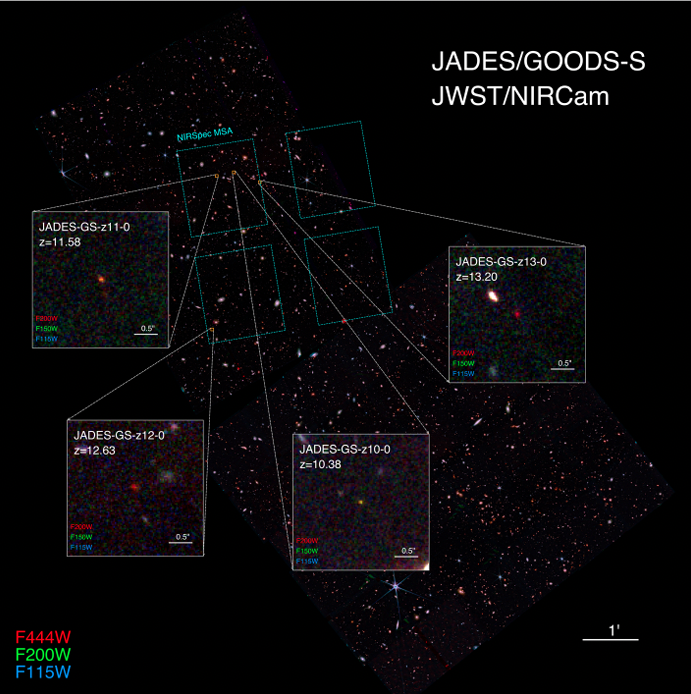
Fig. 122 JWST NIRCam observations of the GOODS-South field in which four \(10 < z < 13\) galaxies have been confirmed from NIRSpec spectroscopy (location of four multi-shutter arrays are shown). Reference: Robertson et al. (2023).

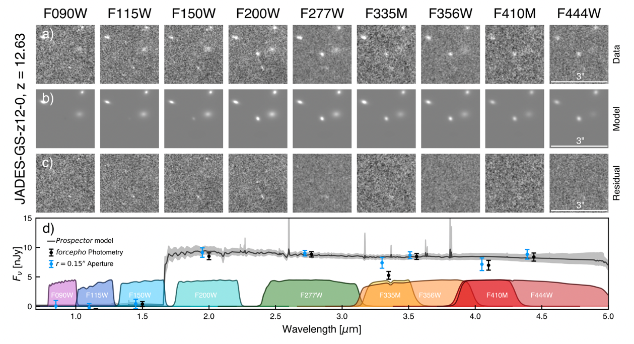
Fig. 123 JWST NIRCam observations of JADES-HS-z12-0 which has been confirmed as a \(z=12.63\) galaxy with NIRSpec. Reference: Robertson et al. (2023).

Exoplanets

Finally, JWST is also helping to characterize exoplanets via spectroscopy. Most observations involve transmission spectroscopy of host stars, from which molecules can be identified in the exoplanet, but in some instances the separation between the parent star and exoplanet is sufficient for direct spectroscopy to be undertaken. For example, Fig. 124 shows JWST NIRSpec and MIRI spectroscopy of VHS 1256b, which is offset by 8 arcsec (150 AU) from its M dwarf host. Spectroscopic features include alkali metals (K, Na), water, methane (CH₄), carbon monoxide and carbon dioxide.

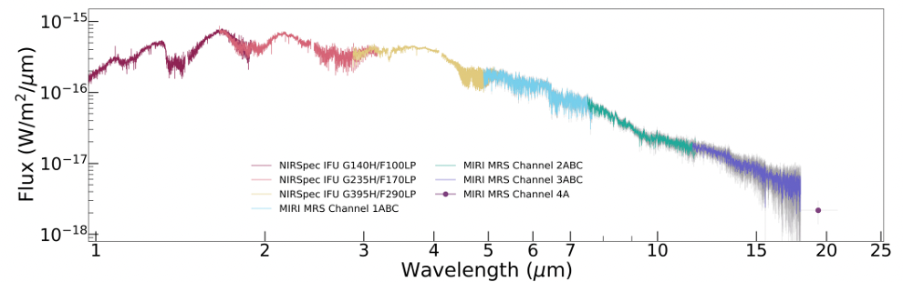
Fig. 124 JWST NIRSpec and MIRI spectroscopy of the planetary-mass companion VHS 1256b to a M dwarf host. Reference: Miles et al. (2023).

Example 5.1

Question

Two nebulae, ionized by identical stars, are observed to have electron temperatures of 9,300K and 11,300 K respectively, with O/H = \(6 \times 10^{-4}\) for the lower temperature nebula. Assuming that gas cools through emission of lines from the two D levels of O⁺ what is the O/H ratio for the hotter nebula?

Solution

Since the nebulae are ionized by identical stars, \(kT_{\ast}\) will be unchanged, and \(y_{O+}\) will be replaced with \(y_{O+}^{\prime}\) in the hotter nebula in Eqn (35). Equating expressions for \(\mathcal{L}_{O+}\) and inserting \(T_{e}\) values including recombiination coefficient (Eqn (33)) leads to \(y_{O+}^{\prime}/y_{O+}\) = 0.45 so for the hotter nebula O/H = \((0.45) (6 \times 10^{-4}) = 2.7 \times 10^{-4}\).

Example 5.2

Question

The 12.8μm line is prominent in the IR spectrum of emission nebulae. This line is identified as the ²P\(_{1/2}\) (upper) to ²P\(_{3/2}\) (lower) fine-structure transition of singly ionized neon. Assuming that this line is collisionally excited, calculate (i) the collisional excitation and de-excitation rates for this transition; (ii) the ratio of Ne⁺ ions in the upper and lower states, if \(T_{e} = 10^{4}\) K, \(n_{e} = 10^{4}\) cm^-3, and the line has a spontaneous decay rate of \(8.6 \times 10^{-3}\) s^-1 and a collisional strength of 0.37.

Solution

\(g_{u} = 4, g_{l} = 2, \chi_{lu}/kT = 0.112\). From Eqn (23), \(C_{lu} = 7.1 \times 10^{-9}\) cm³ s^-1 and \(C_{lu} = 1.6 \times 10^{-8}\) cm³ s^-1. From Eqn (25), \(N_{u}/N_{l} = C_{lu} n_{e}/(C_{ul} n_{e} + A_{ul}) = 123\).

Example 5.3

Question

What is the dynamical age of the nebula associated with He 3-519 shown in Fig. 6 if the distance to the source is 7.1 kpc (from Gaia DR3 parallax)?

Solution

The dynamical age of an expanding nebula is \(\tau_{Dyn} = R/v_{\rm exp}\) where \(R\) is the size of the nebula and \(v_{\rm exp}\) is its expansion velocity. The angular radius of the nebula from the figure is \(\sim\)30 arcsec. For the Gaia-derived distance, \(R \sim 30/206265 \times 7100 = 1.03\) pc or \(3.2 \times 10^{18}\) cm. From Fig. 7, \(v_{\rm sys} \sim 30\) km s^-1 and \(v_{\rm exp} \sim 60\) km s^-1 so \(\tau_{Dyn} = 3.2 \times 10^{18} /6\times 10^{6} = 5.3 \times 10^{11}\) s or 17,000 yr.