\(\renewcommand{\a}{\mathbf{a}}\) \(\renewcommand{\b}{\mathbf{b}}\) \(\renewcommand{\c}{\mathbf{c}}\) \(\newcommand{\g}{\mathbf{g}}\) \(\newcommand{\x}{\mathbf{x}}\) \(\newcommand{\y}{\mathbf{y}}\) \(\newcommand{\z}{\mathbf{z}}\) \(\renewcommand{\r}{\mathbf{r}}\) \(\renewcommand{\v}{\mathbf{v}}\) \(\renewcommand{\u}{\mathbf{u}}\) \(\newcommand{\kk}{\mathbf{k}}\) \(\newcommand{\p}{\mathbf{p}}\) \(\newcommand{\m}{\mathbf{m}}\) \(\renewcommand{\d}{\mathrm{d}}\) \(\newcommand{\e}{\mathrm{e}}\) \(\newcommand{\A}{\mathbf{A}}\) \(\newcommand{\B}{\mathbf{B}}\) \(\newcommand{\D}{\mathbf{D}}\) \(\newcommand{\E}{\mathbf{E}}\) \(\newcommand{\J}{\mathbf{J}}\) \(\newcommand{\F}{\mathbf{F}}\) \(\newcommand{\M}{\mathbf{M}}\) \(\renewcommand{\H}{\mathbf{H}}\) \(\renewcommand{\P}{\mathbf{P}}\) \(\newcommand{\R}{\mathbf{R}}\) \(\renewcommand{\l}{\mathbf{l}}\) \(\renewcommand{\S}{\mathbf{S}}\) \(\newcommand{\V}{\mathbf{V}}\) \(\renewcommand{\L}{\mathbf{L}}\) \(\newcommand{\ms}{\;\text{m}\;\text{s}^{-1}}\) \(\newcommand{\mss}{\;\text{m}\;\text{s}^{-2}}\)
\(\DeclareMathOperator{\sinc}{sinc}\)
\(\newcommand{\kopje}[2]{\vskip0.5em\noindent\textbf{\textsf{{\color{OliveDrab}{Week #1}:}~ #2}}}\) \(\newcommand{\homework}[1]{\noindent{\color{FireBrick}{\textbf{\textsf{Homework:}}} #1}}\) \(\newcommand{\tutorial}[1]{\noindent{\color{SteelBlue}{\textbf{\textsf{Tutorial:}}} #1}}\) \(\newcommand{\problems}[1]{\noindent{\color{LightSlateGrey}{\textbf{\textsf{Weekly problems:}}} #1}}\)
\(\newcommand{\af}[1]{[A\&F: #1]}\) \(\newcommand{\basis}[1]{\hat{\text{\small{e}}}_{#1}}\)
Where do forces come from?#
What is mechanics? It’s not just about projectile motion and pulleys, although there is plenty of that. Mechanics is a way of understanding the behaviour of physical systems. Anything that produces a force can be analysed using mechanics, and that includes gravity, electric and magnetic forces, and even many-body systems like gasses. Only with the development of quantum mechanics did physics truly depart from the framework for understanding Nature that mechanics provided. Relativity, and electric and magnetic fields, can and have all been incorporated into a classical mechanical description.
Mechanics was first cast in the language of forces by Newton in the 1680s, and that was a radical concept at the time, even mystical to some. It was subsequently developed by many others. Laplace introduced differential equations into mechanics in the 1770s, and Hamilton applied the concept of energy to mechanics in the 1820s, developing the language of mechanics as we use it today. Lagrange and Euler developed the calculus of variations for mechanics in the 1750s, which is used equally often in modern physics as an alternative formulation to Hamilton’s.
So what is mechanics? It is a mathematical framework describing the motion of physical systems. It relates the positions and velocities of objects to forces and potentials, and tells us how to calculate how systems behave. It would not be a stretch to claim that the entirety of classical physics falls under the umbrella of mechanics, even though areas like optics and electromagnetism do not simply reduce to the positions and velocities of particles. In this course, we will consider a slightly more modest scope of mechanics as a discipline. We will treat only one, or a few objects at a time, excluding many-body physics. We will not talk about fields, but leave that for second semester. Instead, we bring together the mathematical tools that underpin mechanics.
In this course we will develop the following concepts:
Position, velocity and acceleration as mathematical functions of time,
Forces as vectors and Newton’s laws of motion,
The relation between force, potential, and work.
Most of the course is about developing these techniques, but in the second half we consider the special case of rotating and orbiting bodies. They are incredibly common in physics, and require new concepts such as angular momentum and the moment of inertia. We conclude with the application that started it all for Newton, namely orbital mechanics and the demonstration that Kepler’s laws follow from his inverse-square law of gravity and his three laws of motion.
First, we will ask a simple question: where do forces come from? Let’s consider some simple examples that you are already familiar with.
Worked example: Uniform gravitational acceleration#
When I drop a ball from a (modest) height \(h\), it experiences a force that is directed towards the ground, \(F = mg\), with \(m\) the mass of the ball and \(g=9.81\mss\) the gravitational acceleration. The ball started out at rest, and accelerates towards the ground. What makes the ball `want’ to leave the higher position and move towards the lower position? One answer is that the Earth attracts the ball.
Another, more fruitful answer is that the ball starts out in a position with high potential energy, and it moves towards a position with low potential energy. The force on the ball is in the direction of decreasing potential energy. When we choose the zero point of the potential energy at ground level, the potential energy at height \(h\) is given by
The force \(F=mg\) is in the direction in which the potential energy decreases.
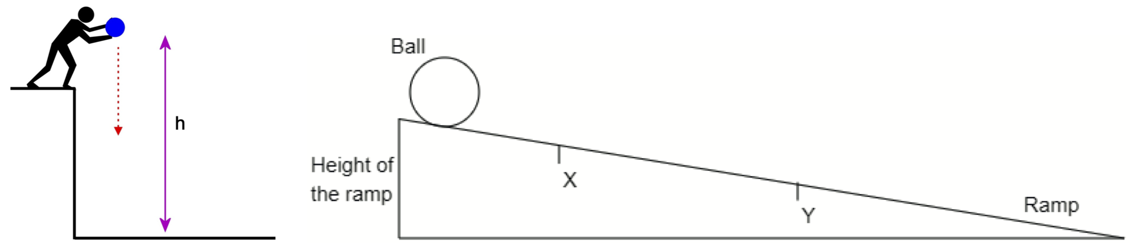
Fig. 1 Left: dropping an object from a height \(h\) to the ground. Right: letting a ball roll from the same height down a ramp.#
Next, imagine we let the ball roll down a ramp (see Fig. 1). If the ramp is very shallow, the force on the ball is quite a bit weaker than when we let it drop straight down. As a result, the ball won’t pick up speed as fast as when we let it drop straight down. The force is proportional to the change in the potential energy.
Worked example: Hooke’s law#
Imagine a spring with a block of mass \(m\) attached to the end. We arrange it horizontally, where the block can slide without friction on a surface. This way we can ignore the role of gravity. The other end of the spring is secured to a fixed point. There is an equilibrium position \(x=0\), where the block is placed such that the spring is neither compressed nor extended. We need to apply a force to move the block, because it will compress or extend the spring. The direction of the compressing/extending force is always away from the equilibrium position \(x=0\). Similarly, from Newton’s third law, the spring exerts a force on the block that is always towards \(x=0\). It is called a restoring force, and because it always points towards \(x=0\), it has a different sign when it is compressing then when it is extending. Moreover, the further the spring is extended, the stronger the restoring force \(F\) on the block:
where \(k\) is the spring constant. This is of course Hooke’s law. The minus sign is very important. It makes the force on the block a restoring force.
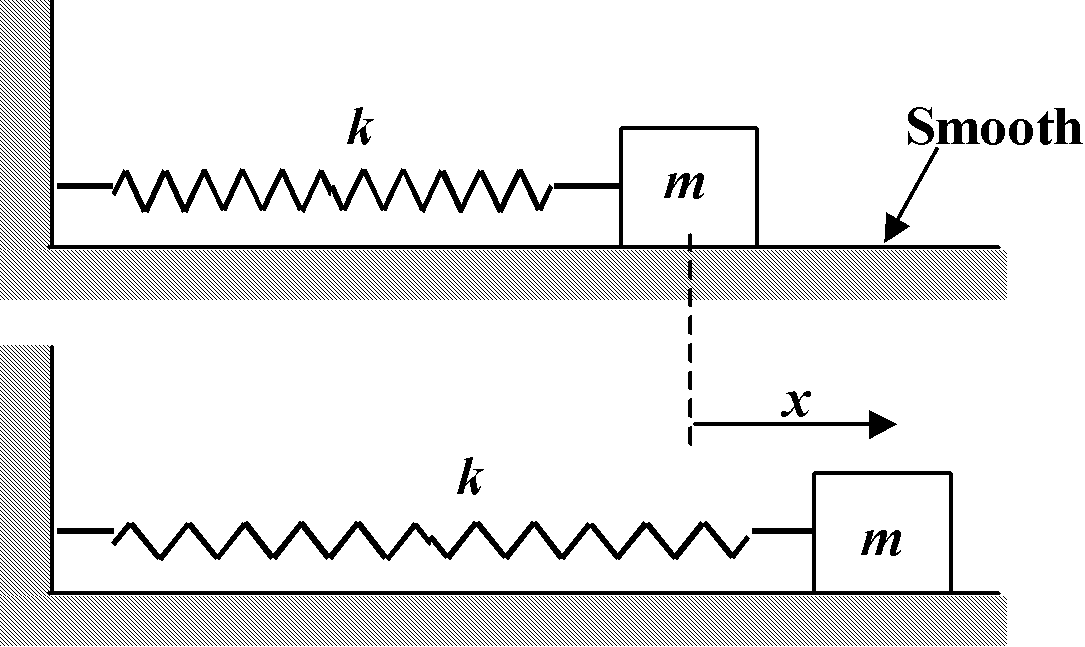
Fig. 2 A black of mass m attached to a spring with spring constant \(k\). The spring is in the equilibrium position in the top figure, with the block position \(x=0\).#
We can also understand this force as a result of a potential. When we compress or extend the spring by an amount \(x\), the potential energy of the system is
It does not matter whether we compress the spring or extend it, the potential energy will be the same, since \((-x)^2 = x^2\). The restoring force on the block is in the direction for which the potential decreases, i.e., in the direction of \(x=0\). So again, the force is given by the change in potential with the distance \(x\). This is given by a derivative of the potential with respect to \(x\). Since the force is in the direction of decreasing potential, it has to be the negative derivative:
(4)#\[F(x) = - \frac{\d V}{\d x}\, .\]
When we substitute the potential \(V_{\rm spring}\), you see that we recover \(F=-kx\). Note that all the signs for \(F\) are correct, both for positive and negative \(x\).
Note that we can add a constant \(V_0\) to the potential, and it will not contribute to the force, since the derivative of a constant is zero. This means that we can pick the zero point of our potential wherever we want, without observable consequences for the force. We already used this in the first example, when we chose \(V=0\) at ground level. We tend to pick the zero point of \(V\) in such a way that it makes our analysis simplest.
At this point it is worth drawing attention to the way we use mathematics in physics. When you see an expression like equation (4), you should treat both \(F\) and \(V\) as a function of \(x\). The specific labels/names of functions (here \(F\) and \(V\)) are not important for how we manipulate those functions mathematically (e.g., in differentiation, integration, etc.). We \emph{need} to give different functions different names based on the physical quantities they represent (force \(F\) and potential \(V\)). Sometimes we will explicitly state the variables \((x)\), such as \(F(x)\) or \(V(x)\), while at other times we will not. Typically, if we include the functional dependence it will be on the left-hand side—as in equation (4)—to remind us what variable we are interested in. Previously, you may have taken derivatives almost exclusively on functions called \(f(x)\) or \(y(x)\). Now you have to extrapolate this to other letters. In your degree you will take derivatives more than doing any other mathematical operation, so make sure you that by the end of the semester are completely comfortable with the procedure, especially including the chain rule and product rule.
Worked example: Newton’s law of gravity#
Newton’s famous insight was that the force that pulls apples to Earth is the same that makes the moon orbit the Earth. The constant gravitational acceleration \(g\) is only an approximation for when the drop height \(h\) is small compared to the radius of the Earth. The force on a mass \(m\) due to another mass \(M\) obeys Newton’s inverse-square law of gravity:
where \(G= 6.67408 \times 10^{-11}~{\rm m}^3\; {\rm kg}^{-1}\; {\rm s}^{-2}\) is Newton’s constant of gravitation. We included a minus sign, because the force of gravity is attractive. The force lies in the direction along the axis that connects the two masses.
We can also cast this problem in terms of potential energy. The closer that the mass \(m\) is to mass \(M\), the lower its potential energy. We define \(V=0\) for the situation where the two masses are infinitely far apart, and we can write the potential as
The direction in which the potential changes is \(r\). So if we want to find the force, we need to take the derivative in the \(r\) direction:
which agrees with equation (5). Note that we take the derivative with respect to \(r\), not \(x\). In general we will have to be careful about the direction in which the potential has its steepest descent, because that is where the force will be directed. The steepest descent is exactly the direction a ball will roll on a map with uneven elevation (for example rolling down a hill).
Worked example: Electrostatic force between two charges#
As a final example of forces between objects, consider two charges, \(q_1\) and \(q_2\) a distance \(d\) apart. The force on charge \(q_1\) due to charge \(q_2\) is given by
where \(\epsilon_0\) is the permittivity of free space. Even though we wrote a distance \(d\), this is essentially again an inverse-square law, and it makes sense to use the coordinate \(r\) instead of \(d\). The force is again directed along the axis connecting the two charges, and to a large degree the connection with the electric potential energy is very similar to that of the two masses in Newton’s law of gravity:
The one notable difference is the lack of the minus sign. In gravity, all the masses are positive numbers, whereas charges can be both positive and negative. This potential says that when two charges have different signs, the overall potential is negative and they attract each other. When the charges have equal sign the potential is positive and the charges repel. You can verify that we obtain the correct electrostatic force when we take the negative derivative with respect to \(r\):
Again, the force is in the direction of the steepest descent.
There are a number of things to note here:
The force is in the direction of the steepest descent, and therefore force is a vector while the potential is a scalar. We have not shown this systematically in our equations so far, but it is important to keep in mind that we deal with vectors.
The sign of the force is important; this is just the one-dimensional aspect of the fact that a force is a vector. Don’t ignore it!
Not all forces can be written as derivatives of a potential, most notably friction forces don’t have a potential, and magnetic forces have a much more complicated potential that we will not discuss here. These forces are still important, but we will have to deal with them in other ways.