\(\renewcommand{\a}{\mathbf{a}}\) \(\renewcommand{\b}{\mathbf{b}}\) \(\renewcommand{\c}{\mathbf{c}}\) \(\newcommand{\g}{\mathbf{g}}\) \(\newcommand{\x}{\mathbf{x}}\) \(\newcommand{\y}{\mathbf{y}}\) \(\newcommand{\z}{\mathbf{z}}\) \(\renewcommand{\r}{\mathbf{r}}\) \(\renewcommand{\v}{\mathbf{v}}\) \(\renewcommand{\u}{\mathbf{u}}\) \(\newcommand{\kk}{\mathbf{k}}\) \(\newcommand{\p}{\mathbf{p}}\) \(\newcommand{\m}{\mathbf{m}}\) \(\renewcommand{\d}{\mathrm{d}}\) \(\newcommand{\e}{\mathrm{e}}\) \(\newcommand{\A}{\mathbf{A}}\) \(\newcommand{\B}{\mathbf{B}}\) \(\newcommand{\D}{\mathbf{D}}\) \(\newcommand{\E}{\mathbf{E}}\) \(\newcommand{\J}{\mathbf{J}}\) \(\newcommand{\F}{\mathbf{F}}\) \(\newcommand{\M}{\mathbf{M}}\) \(\renewcommand{\H}{\mathbf{H}}\) \(\renewcommand{\P}{\mathbf{P}}\) \(\newcommand{\R}{\mathbf{R}}\) \(\renewcommand{\l}{\mathbf{l}}\) \(\renewcommand{\S}{\mathbf{S}}\) \(\newcommand{\V}{\mathbf{V}}\) \(\renewcommand{\L}{\mathbf{L}}\) \(\newcommand{\ms}{\;\text{m}\;\text{s}^{-1}}\) \(\newcommand{\mss}{\;\text{m}\;\text{s}^{-2}}\)

\(\DeclareMathOperator{\sinc}{sinc}\)

\(\newcommand{\kopje}[2]{\vskip0.5em\noindent\textbf{\textsf{{\color{OliveDrab}{Week #1}:}~ #2}}}\) \(\newcommand{\homework}[1]{\noindent{\color{FireBrick}{\textbf{\textsf{Homework:}}} #1}}\) \(\newcommand{\tutorial}[1]{\noindent{\color{SteelBlue}{\textbf{\textsf{Tutorial:}}} #1}}\) \(\newcommand{\problems}[1]{\noindent{\color{LightSlateGrey}{\textbf{\textsf{Weekly problems:}}} #1}}\)

\(\newcommand{\af}[1]{[A\&F: #1]}\) \(\newcommand{\basis}[1]{\hat{\text{e}}_{#1}}\)

Orbital mechanics

We now arrive at the capstone of this lecture series: Kepler’s laws of planetary motion. They can be stated as follows:

1. Planets orbit the Sun in elliptical orbits.

2. The planet sweeps out equal areas in equal time.

3. The orbital period squared is proportional to the semi-major axis cubed.

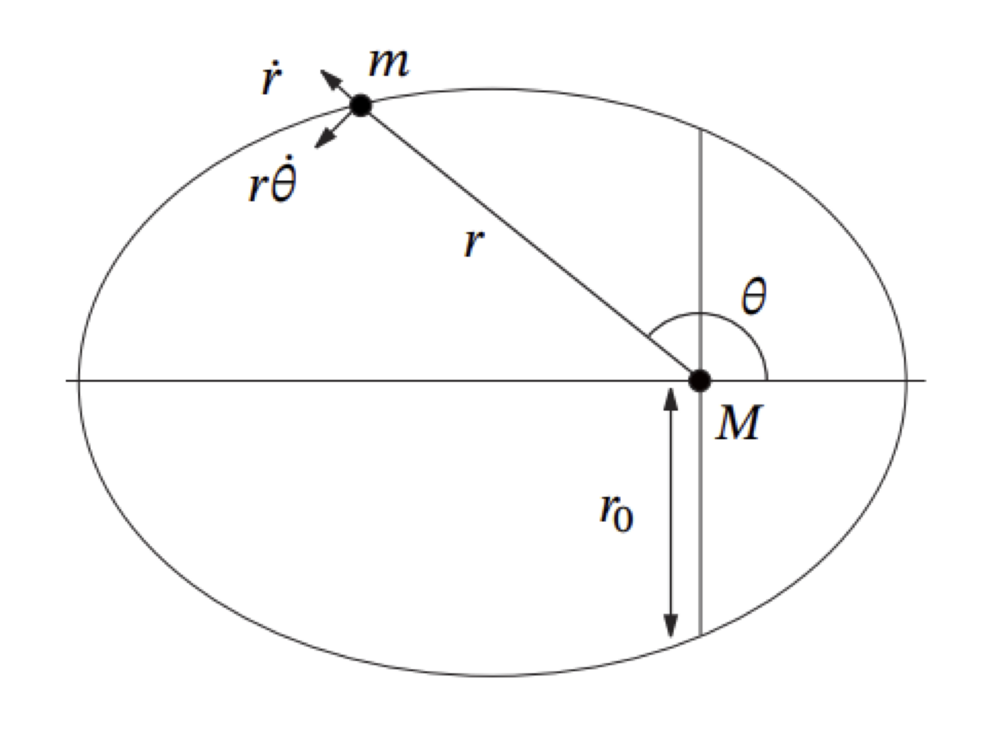
Fig. 17 A planet of mass \(m\) orbiting on an elliptical path around a larger mass \(M\). The distance between the two masses changes throughout the orbit. The velocity of the small mass is resolved into two components, one pointing radially and the other perpendicular to this.

We will prove these laws in turn, but first we need to explore the mathematics of ellipses in more detail. An elliptical orbit in cartesian coordinates is given by

(96)\[\begin{align} \frac{x^2}{a^2} + \frac{y^2}{b^2} = 1\, , \end{align}\]

where \(a\) and \(b\leq a\) are the semi-major and semi-minor axes, respectively. It is convenient to define the eccentricity of the ellipse \(e\) as a measure of how the shape of the ellipse deviates from a circle:

(97)\[\begin{align} e = \sqrt{1-\frac{b^2}{a^2}} \qquad\text{with}\qquad 0\leq e \leq 1\, . \end{align}\]

When \(e=0\) the ellipse is a circle (i.e., the deviation from a circle is zero), and when \(e=1\) the ellipse is a line segment.

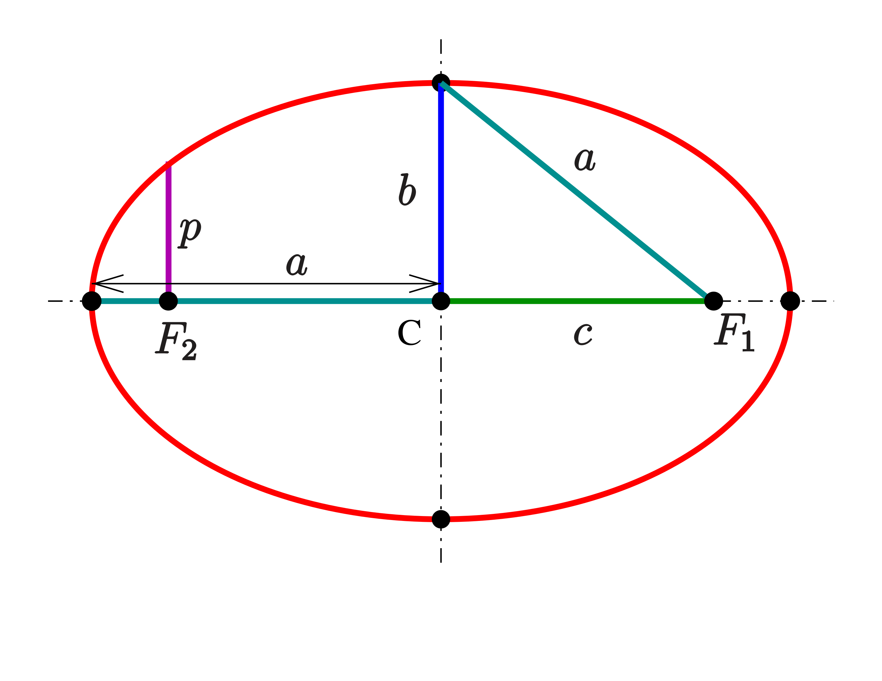
Fig. 18 The ellipse: Here, \(c=\sqrt{a^2-b^2}\), such that \(e = c/a\).

Since we are solving the problem of planetary motion in polar coordinates, we need to express the ellipse in terms of \(r\) and \(\theta\). Using \(x=r\cos\theta\) and \(y=r\sin\theta\), we find that

(98)\[\begin{align} r(\theta) = \frac{b^2/a}{1+e \cos\theta}\, . \end{align}\]

The origin coincides with one of the foci (\(F_1\) or \(F_2\) in figure 18) of the ellipse.

Kepler’s First Law

For Kepler’s first law, we want to show that the orbit of a planet is an ellipse, namely

(99)\[\begin{align} r(\theta) = \frac{b^2/a}{1+e \cos\theta}\, , \end{align}\]

for some values of \(a\), \(b\), and \(e\) that we need to determine. We start with the energy in equation (95) and determine the force in the radial direction from the potential \(V_{\rm eff}\):

(100)\[\begin{align} F = m \ddot{r} = - \frac{\d V_{\rm eff}}{\d r} = \frac{L^2}{mr^3} - \frac{GmM}{r^2}\, . \end{align}\]

We can divide by \(m\) and reintroduce \(\dot{\theta} = L/mr^2\) to obtain

(101)\[ \ddot{r} = r \dot{\theta}^2 - \frac{GM}{r^2}\, .\]

This is not a differential equation we can easily solve, but fortunately we can cast it in a much more amenable form. If we make the substitution \(\rho = 1/r\), we can write

(102)\[\begin{align} \frac{\d\rho}{\d\theta} = \frac{\d}{\d\theta}\frac{1}{r} = -\frac{1}{r^2} \frac{\d r}{\d\theta} = -\frac{1}{r^2} \dot{r} \frac{\d t}{\d\theta} = -\frac{m\dot{r}}{L}\, . \end{align}\]

However, equation (101) requires the second time derivative \(\ddot{r}\). We can get this via a circuitous way, namely from the second derivative of \(\rho\) with respect to \(\theta\):

(103)\[\begin{align} \frac{\d^2\rho}{\d\theta^2} = -\frac{\d}{\d\theta}\frac{m\dot{r}}{L} = -\frac{m}{L} \frac{\d \dot{r}}{\d\theta} = -\frac{m}{L} \ddot{r} \frac{\d t}{\d\theta} = -\frac{m^2 r^2}{L^2} \ddot{r}\, . \end{align}\]

We can solve for \(\ddot{r}\) and substitute this into equation (101). This leads to

(104)\[\begin{align} -\frac{L^2 \rho^2}{m^2} \frac{\d^2\rho}{\d\theta^2} = \frac{L^2 \rho^3}{m^2} - GM\rho^2\, . \end{align}\]

Dividing this equation by \(\rho^2 L^2/m^2\), we obtain the differential equation:

(105)\[\begin{align} \frac{\d^2\rho}{\d\theta^2} + \rho - \frac{GMm^2}{L^2} = 0\, , \end{align}\]

This is mathematically identical to the differential equation for a harmonic oscillator, whose solutions can be written as

(106)\[\begin{align} \rho(\theta) = \frac{GMm^2}{L^2} + B \cos(\theta+\phi_0)\, , \end{align}\]

where \(B\) is the `amplitude’ of the solution, and we can set \(\phi_0 = 0\) as our initial condition. Solving for \(r(\theta) = 1/\rho(\theta)\), we find

(107)\[\begin{align} r(\theta) = \frac{L^2/Gm^2M}{1+L^2 B/Gm^2M \cos\theta}\, . \end{align}\]

This is an elliptical orbit with

(108)\[ e = \frac{L^2 B}{Gm^2M} \qquad\text{and}\qquad \frac{b^2}{a} = \frac{L^2}{Gm^2M}\, .\]

This proves Kepler’s first law. The eccentricity becomes zero for \(B=0\), or where \(\rho\) is a constant for all angles \(\theta\).

Kepler’s Second Law

From the conservation of angular momentum and equation (64) we know that

(109)\[\begin{align} r^2 \dot{\theta} = \frac{L}{m} = \text{constant.} \end{align}\]

However, \(r^2 \dot{\theta}\) has a clear geometric meaning, as shown in Fig. 19. The shaded area is a triangle when \(r\d\theta\) is infinitesimally small, and the area of this triangle is

(110)\[\begin{align} \d A = \frac12 r\, r \d\theta = \frac12 r^2\d\theta\, . \end{align}\]

Therefore,

(111)\[\begin{align} \frac{\d A}{\d t} = \frac12 r^2 \dot{\theta} = \text{constant.} \end{align}\]

In other words, the rate of the area \(A\) swept out by the line connecting the planet and the origin is constant over time, and this is precisely Kepler’s second law. You see that it is an expression of the conservation of angular momentum.

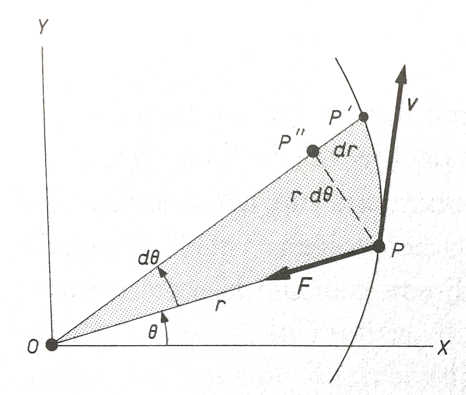
Fig. 19 The area of the shaded triangle is \(\simeq\frac12 r\, r \d\theta\).

Kepler’s Third Law

The area of an ellipse is \(\pi ab\), and the rate of sweeping out area in elliptical orbits is a constant \(L/2m\). The time \(T\) to complete an orbit is equal to the area divided by the rate of area swept. In other words,

(112)\[ T = \dfrac{\pi ab}{{L/2m}}= \dfrac{2m\pi ab}{L}\, .\]

We now need to relate \(T\) to the semi-major axis \(a\). This is quite straightforward if we extract \(b\) from equation (108) and use it to eliminate \(b\) from equation (112).

From equations (108) and (112) we see that \(b^2\) is equal to

(113)\[\begin{align} b^2 = \frac{a L^2}{Gm^2M} = \frac{T^2 L^2}{4m^2\pi^2a^2}\, . \end{align}\]

Hence

(114)\[\begin{align} \frac{a L^2}{Gm^2M} = \frac{T^2 L^2}{4m^2\pi^2a^2} \qquad\text{or}\qquad \frac{T^2}{a^3} = \frac{4\pi^2}{GM} = \text{constant}\, . \end{align}\]

This proves Kepler’s third law.

---

The derivation of Kepler’s laws was a triumph for Newtonian mechanics. It demonstrated that the inverse-square law of gravity was capable of reproducing Kepler’s experimentally well-established laws from simple principles (Newton’s three laws), even though the application of Newton’s laws is not necessarily all that straightforward. The conservation of energy and angular momentum played a central role in understanding where Kepler’s laws come from.

Mechanics is a very mathematical subject that requires familiarity with derivatives and integrals, vectors, and non-cartesian coordinate systems. However, mechanics lies at the heart of all classical physics, and these techniques are a prerequisite for understanding a wide range of topics further in your studies.