\(\renewcommand{\a}{\mathbf{a}}\) \(\renewcommand{\b}{\mathbf{b}}\) \(\renewcommand{\c}{\mathbf{c}}\) \(\newcommand{\g}{\mathbf{g}}\) \(\newcommand{\x}{\mathbf{x}}\) \(\newcommand{\y}{\mathbf{y}}\) \(\newcommand{\z}{\mathbf{z}}\) \(\renewcommand{\r}{\mathbf{r}}\) \(\renewcommand{\v}{\mathbf{v}}\) \(\renewcommand{\u}{\mathbf{u}}\) \(\newcommand{\kk}{\mathbf{k}}\) \(\newcommand{\p}{\mathbf{p}}\) \(\newcommand{\m}{\mathbf{m}}\) \(\renewcommand{\d}{\mathrm{d}}\) \(\newcommand{\e}{\mathrm{e}}\) \(\newcommand{\A}{\mathbf{A}}\) \(\newcommand{\B}{\mathbf{B}}\) \(\newcommand{\D}{\mathbf{D}}\) \(\newcommand{\E}{\mathbf{E}}\) \(\newcommand{\J}{\mathbf{J}}\) \(\newcommand{\F}{\mathbf{F}}\) \(\newcommand{\M}{\mathbf{M}}\) \(\renewcommand{\H}{\mathbf{H}}\) \(\renewcommand{\P}{\mathbf{P}}\) \(\newcommand{\R}{\mathbf{R}}\) \(\renewcommand{\l}{\mathbf{l}}\) \(\renewcommand{\S}{\mathbf{S}}\) \(\newcommand{\V}{\mathbf{V}}\) \(\renewcommand{\L}{\mathbf{L}}\) \(\newcommand{\ms}{\;\text{m}\;\text{s}^{-1}}\) \(\newcommand{\mss}{\;\text{m}\;\text{s}^{-2}}\)

\(\DeclareMathOperator{\sinc}{sinc}\)

\(\newcommand{\kopje}[2]{\vskip0.5em\noindent\textbf{\textsf{{\color{OliveDrab}{Week #1}:}~ #2}}}\) \(\newcommand{\homework}[1]{\noindent{\color{FireBrick}{\textbf{\textsf{Homework:}}} #1}}\) \(\newcommand{\tutorial}[1]{\noindent{\color{SteelBlue}{\textbf{\textsf{Tutorial:}}} #1}}\) \(\newcommand{\problems}[1]{\noindent{\color{LightSlateGrey}{\textbf{\textsf{Weekly problems:}}} #1}}\)

\(\newcommand{\af}[1]{[A\&F: #1]}\) \(\newcommand{\basis}[1]{\hat{\text{e}}_{#1}}\)

Angular momentum

Let’s consider again the torque in vector form given in the previous lecture:

(54)\[\begin{align} \vec{\tau} = \r\times \F = \r\times \frac{\d\p}{\d t}\, . \end{align}\]

We can write the time derivative of \(\p\) in terms of the chain rule on the whole cross product \(\r\times\p\) using

(55)\[\begin{align} \frac{\d}{\d t} (\r\times\p) = \frac{\d\r}{\d t} \times \p + \r\times \frac{\d\p}{\d t}\, . \end{align}\]

The term \(\dot{\r}\times \p\) is zero because \(\dot{\r}=\v\) and \(\p =m\v\) are parallel, and we can therefore write

(56)\[\begin{align} \tau = \frac{\d }{\d t} (\r\times\p) \equiv \frac{\d \L}{\d t} \qquad\text{with}\qquad \L = \r\times\p\, . \end{align}\]

The quantity \(\L\) is called angular momentum, and it is the rotational equivalent to the linear momentum \(\p\). The expression \(\vec{\tau} = \dot{\L}\) is the analog of \(\F = \dot{\p}\) for rotational motion.

Just like the case where an absence of external forces leads to conservation of momentum:

(57)\[\begin{align} \F = 0 = \frac{\d\p}{\d t} \qquad\Rightarrow\qquad \p ~\text{is constant in time,} \end{align}\]

so does an absence of torque lead to conservation of angular momentum:

(58)\[\begin{align} \vec{\tau} = 0 = \frac{\d\L}{\d t} \qquad\Rightarrow\qquad \L ~\text{is constant in time.} \end{align}\]

One example of this is planetary motion. The only force on a planet orbiting a star is gravity, which always points along the line connecting the planet and the star at every moment in time. Therefore, the cross product \(\r\times\F = \vec{\tau}\) is always zero (\(\F\) is in the direction of \(\r\)). As a consequence, the angular momentum of a planet in orbit around a star is conserved. Specifically the angular momentum at the aphelion is equal to the angular momentum at the perihelion:

(59)\[\begin{align} \L = \r_{\rm ap} \times \p_{\rm ap} = \r_{\rm peri} \times \p_{\rm peri}\, . \end{align}\]

At both aphelion and perihelion the position and momentum vectors are perpendicular, so we can ignore the \(\sin\theta\) term in the cross product. We then have

(60)\[\begin{align} r_{\rm ap} p_{\rm ap} = r_{\rm peri} p_{\rm peri}\, , \end{align}\]

where we use the convention that non-bold symbols signify the magnitude.

It is because of this conservation law that angular momentum is so important and ubiquitous in physics. The orbital motion of electrons in atoms is classified by energy and angular momentum, and the entire periodic table is a direct consequence of the allowed energy and angular momentum values of the electrons. Rotating black holes have angular momentum, and this creates interesting frame dragging effects near their horizons. Gyroscopes keep their orientation in space because of conservation of angular momentum, and this allows for navigation at sea in the absence of external signals (such as the position of the stars on cloudy nights). These are just a few examples of the central importance of angular momentum in physics. You will keep encountering this topic throughout your studies.

---

The expression \(\L = \r\times\p\) depends explicitly on \(\r\), and therefore \(\L\) must always be given relative to the coordinate origin of \(\r\). Often the choice of origin is so obvious that people don’t specify it, but you should always make sure that you know which origin is used to calculate the angular momentum. In atomic and planetary systems it is typically the centre of mass.

As an example, let’s consider simple circular motion, where \(\r\) is the position vector of a particle of mass \(m\) moving in a circle around the origin, and \(\p\) is the momentum that is directed in the tangent direction to the circle. The origin of \(\r\) is the centre of the circle. Since \(\r\) and \(\p\) are perpendicular, we can write the magnitude of \(\L=\r\times\p\) as

(61)\[ L = rp = mrv = mr^2\omega\, ,\]

where we preferred \(\omega\) to \(v\) because the angular velocity is more natural to use here (\(v = r\omega\)). From the cross product we deduce that \(\L\) is in the same direction as \(\vec{\omega}\), so we can write

(62)\[\begin{align} \L = mr^2\vec{\omega}\, . \end{align}\]

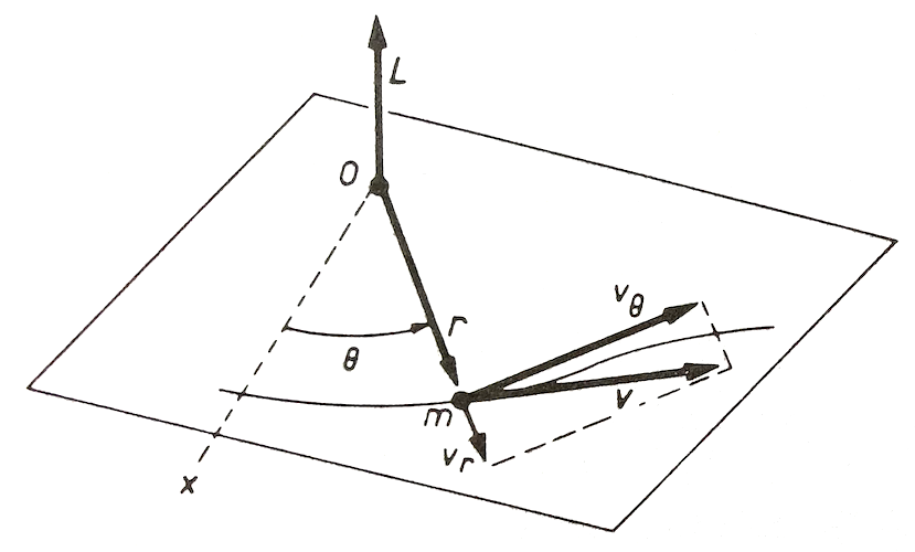
Fig. 15 Angular momentum of a particle moving along a general curved path.

Next, consider a more general curved motion, shown in Fig. 16. At any point along the path the velocity \(\v\) will have a radial and a transversal component, \(\v_r\) and \(\v_\theta\), which sum together to form \(\v = \v_r + \v_\theta\). The angular momentum can then be written as

(63)\[\begin{align} \L = \r\times\p = m \r\times \v = m \r\times (\v_r + \v_\theta) = m \r\times \v_r + m\r\times \v_\theta = m\r\times \v_\theta\, . \end{align}\]

The last equality holds because \(\v_r\) is parallel to \(\r\), by definition, and the cross product between the two must therefore be zero. Hence \(\L\) always captures only the transversal part of the momentum. Also, since \(v_\theta = r \d\theta/\d t\), we can write the magnitude in the most general form

(64)\[L = mr^2\frac{\d\theta}{\d t}\, .\]

When the angular velocity is constant, this reduces to equation (61).

Another consequence of the conservation of angular momentum is that the direction of \(\L\) does not change. This means that the motion must be confined to a plane perpendicular to \(\L\). Translating this to the orbital motion of planets, each planet must always move in a plane. Without external disturbances, no planet can drift out of this plane as it orbits the Sun.

---

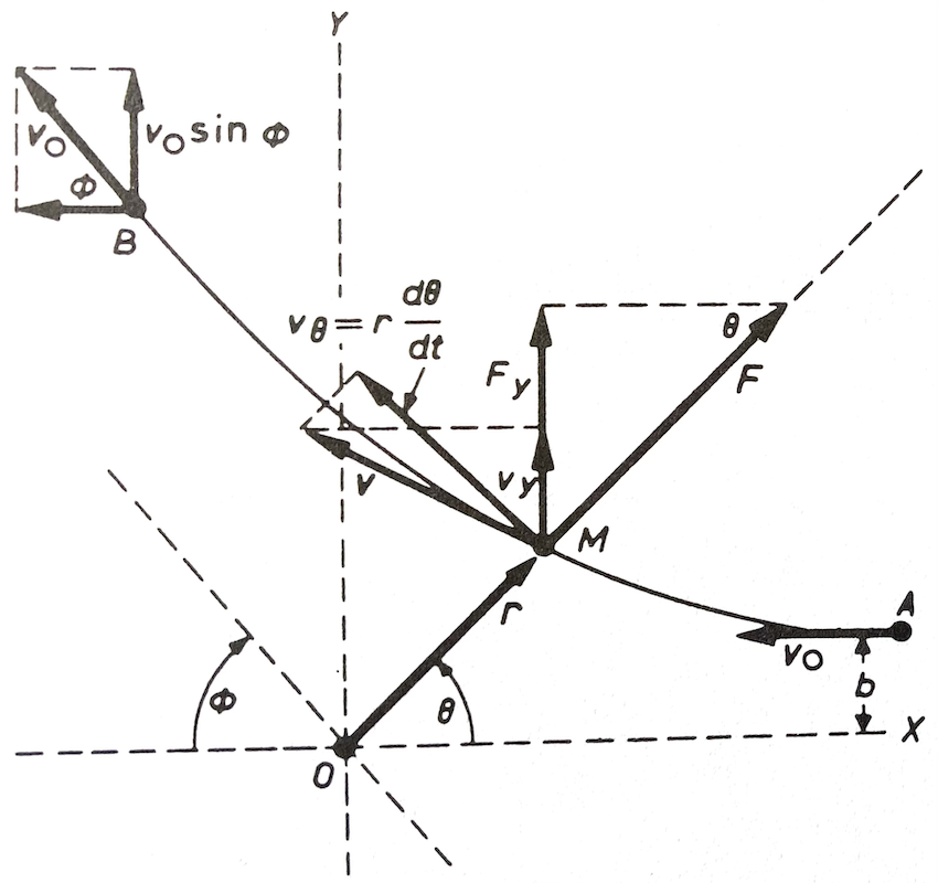
Fig. 16 Scattering from a \(1/r\) potential

Finally, we consider the important example of the scattering of particles from a central potential, shown in Fig. 17. We assume that the central potential falls off with \(1/r\) (for example the electrostatic potential of a point charge), so that the force is given by \(F = k/r^2\). We want to know how the scattering angle \(\phi\) depends on the scattering parameter \(b\), the mass \(m\) of the particle, and its initial velocity \(v_0\). First, we calculate the angular momentum of the particle. In point \(A\) in Fig. 17, the angular momentum is (see weekly practice problems):

(65)\[\begin{align} L = m v_0 b\, . \end{align}\]

Then, at some other (arbitrary) point \(M\), according to equation (64) the angular momentum must be equal to

(66)\[\begin{align} L = m r^2 \frac{\d\theta}{\d t}\, . \end{align}\]

Conservation of angular momentum applies, since \(F\) is a central force, so

(67)\[ m r^2 \frac{\d\theta}{\d t} = m v_0 b\, .\]

Next, we consider the vertical force

(68)\[\begin{align} m \frac{\d v_y}{\d t} = F_y = F\sin\theta = \frac{k\sin\theta}{r^2}\, . \end{align}\]

This allows us to eliminate \(r^2\) from equation (67):

(72)\[ \frac{\d v_y}{\d t} = \frac{k\sin\theta}{mv_0 b} \frac{\d\theta}{\d t} \, .\]

As the particle comes in from \(t\to-\infty\), scatters, and whizzes off to \(t\to+\infty\), it changes direction from a horizontal trajectory to an asymptotic trajectory at an angle \(\phi\). We can therefore integrate both sides of equation (72) from the initial value of \(v_y\) and \(\theta\) to their final values:

(72)\[ \int_0^{v_0\sin\phi} \d v_y = \frac{k}{mv_0 b} \int_0^{\pi-\phi}\sin\theta\,\d\theta\, .\]

Note the limits of integration: as time runs from \(-\infty\) to \(+\infty\), the vertical component of the velocity \(v_y\) goes from zero to \(v_0\sin\phi\), and the angle \(\theta\) goes from zero to \(\pi-\phi\) (see Fig. 17). Solving these integrals is straightforward, and yields

(72)\[ v_0\sin\phi = \frac{k}{mv_0 b} (1+\cos\phi)\, .\]

Extracting \(\phi\) from this is not entirely trivial, but can be done using the cotangens:

(72)\[ \cot\frac{\phi}{2} = \frac{mv_0^2 b}{k}\, .\]

Hence the potential \(V = k/r\) predicts a very specific scattering angle for the various velocities \(v_0\) and scattering parameters \(b\). A different potential, for example \(V=k/r^n\), would have given rise to a different relationship between the scattering angle and \(v_0\) and \(b\). This is why scattering experiments are used in particle physics to understand the inner workings of subatomic particles. It allowed Rutherford to deduce from his scattering experiments that the atom consists of a massive nucleus surrounded by light electrons.

A note on energy conservation: We could not solve this problem using energy conservation, since the balance between kinetic and potential energy depends on the distance of the particle to the centre of the potential. Energy is still conserved, but here it did not give us all the information we needed. This underscores the importance of angular momentum.