\(\renewcommand{\a}{\mathbf{a}}\) \(\renewcommand{\b}{\mathbf{b}}\) \(\renewcommand{\c}{\mathbf{c}}\) \(\newcommand{\g}{\mathbf{g}}\) \(\newcommand{\x}{\mathbf{x}}\) \(\newcommand{\y}{\mathbf{y}}\) \(\newcommand{\z}{\mathbf{z}}\) \(\renewcommand{\r}{\mathbf{r}}\) \(\renewcommand{\v}{\mathbf{v}}\) \(\renewcommand{\u}{\mathbf{u}}\) \(\newcommand{\kk}{\mathbf{k}}\) \(\newcommand{\p}{\mathbf{p}}\) \(\newcommand{\m}{\mathbf{m}}\) \(\renewcommand{\d}{\mathrm{d}}\) \(\newcommand{\e}{\mathrm{e}}\) \(\newcommand{\A}{\mathbf{A}}\) \(\newcommand{\B}{\mathbf{B}}\) \(\newcommand{\D}{\mathbf{D}}\) \(\newcommand{\E}{\mathbf{E}}\) \(\newcommand{\J}{\mathbf{J}}\) \(\newcommand{\F}{\mathbf{F}}\) \(\newcommand{\M}{\mathbf{M}}\) \(\renewcommand{\H}{\mathbf{H}}\) \(\renewcommand{\P}{\mathbf{P}}\) \(\newcommand{\R}{\mathbf{R}}\) \(\renewcommand{\l}{\mathbf{l}}\) \(\renewcommand{\S}{\mathbf{S}}\) \(\newcommand{\V}{\mathbf{V}}\) \(\renewcommand{\L}{\mathbf{L}}\) \(\newcommand{\ms}{\;\text{m}\;\text{s}^{-1}}\) \(\newcommand{\mss}{\;\text{m}\;\text{s}^{-2}}\)

\(\DeclareMathOperator{\sinc}{sinc}\)

\(\newcommand{\kopje}[2]{\vskip0.5em\noindent\textbf{\textsf{{\color{OliveDrab}{Week #1}:}~ #2}}}\) \(\newcommand{\homework}[1]{\noindent{\color{FireBrick}{\textbf{\textsf{Homework:}}} #1}}\) \(\newcommand{\tutorial}[1]{\noindent{\color{SteelBlue}{\textbf{\textsf{Tutorial:}}} #1}}\) \(\newcommand{\problems}[1]{\noindent{\color{LightSlateGrey}{\textbf{\textsf{Weekly problems:}}} #1}}\)

\(\newcommand{\af}[1]{[A\&F: #1]}\) \(\newcommand{\basis}[1]{\hat{\text{e}}_{#1}}\)

Applications

In this lecture we will consider a few applications of the basic concepts of mechanics that we have covered so far, and show the broad applicability of the theory.

---

Van der Waals forces between atoms

The Lennard-Jones potential, shown in Fig. 8, describes the Van der Waals potential energy between two atoms,

(11)\[\begin{align} V(r) = - \epsilon \left[2\left( \frac{r_{\rm m}}{r}\right)^6 - \left( \frac{r_{\rm m}}{r}\right)^{12} \right]\, , \end{align}\]

where \(r\) is the distance between the molecules, and \(-\epsilon\) is the bottom of the potential well at a distance \(r_{\rm m}\). This is a very complicated potential, but we can solve for the situation when the two atoms are roughly a distance \(r_{\rm m}\) apart. In this case the two atoms are bound together since they are in the potential well.

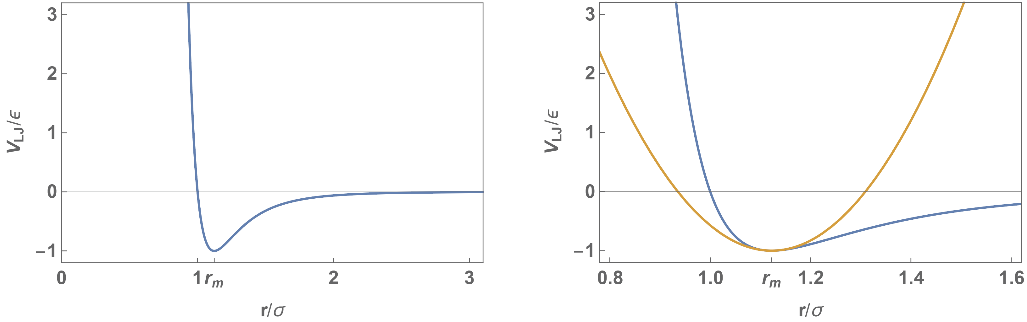
Fig. 6 The Lennard-Jones potential. Left: the potential with minimum at \(r_{\rm m}\). Right: the parabolic approximation of the Lennard-Jones potential around \(r_{\rm m}\) that leads to a linear restoring force.

A slight change in distance between them will increase the potential energy, and there will be a force restoring the atoms to a distance \(r_{\rm m}\). We find the force from

(12)\[\begin{align} F(r) = -\frac{\d V}{\d r} = -12 \epsilon \left[ \frac{r_{\rm m}^6}{r^7} - \frac{r_{\rm m}^{12}}{r^{13}} \right]\, . \end{align}\]

This is still far too complicated to substitute into Newton’s law, so we will approximate this force with a Taylor series around \(r_{\rm m}\), where we are interested in the physical behaviour of the atoms:

(13)\[\begin{align} F(r) = F(r_{\rm m}) + (r-r_{\rm m}) \left.\frac{\d F}{\d r}\right|_{r=r_{\rm m}} + \frac{(r-r_{\rm m})^2}{2} \left.\frac{\d^2 F}{\d r^2}\right|_{r=r_{\rm m}} + \ldots \end{align}\]

We can take the derivatives of \(F\) with respect to \(r\) and substitute \(r=r_{\rm m}\):

(14)\[\begin{align} F(r_{\rm m}) = 0 \qquad\text{and}\qquad \left.\frac{\d F}{\d r} \right|_{r=r_{\rm m}} = -12 \epsilon \left(\frac{13 r_{\rm m}^{12}}{r^{14}}-\frac{7 r_{\rm m}^6}{r^8}\right)_{r=r_{\rm m}} = -\frac{72 \epsilon}{r_{\rm m}^2} \end{align}\]

We need the force only up to the first non-zero term, the linear term. This corresponds to the quadratic potential around \(r_{\rm m}\):

(15)\[\begin{align} F(r) \simeq -(r-r_{\rm m}) \frac{72 \epsilon}{r_{\rm m}^2}\, . \end{align}\]

We can define \(k=72 \epsilon/r_{\rm m}^2\) and the radial displacement from the equilibrium position \(x = r-r_{\rm m}\). The force is then in a form that we can use in Newton’s second law:

(16)\[\begin{align} F(x) \simeq -kx\, . \end{align}\]

This is formally identical to Hooke’s law, and the solutions to the differential equation are therefore given by equation fvmnghre9w4ueirdfg. The two atoms thus oscillate harmonically towards and away from each other around the equilibrium separation \(r_{\rm m}\).

---

Lifting heavy loads

Consider a system with two pulleys as shown in the figure below. Calculate the force needed to lift a load with mass \(m\) using this pulley system. You will need to consider the acceleration of the load for the two coordinates \(x\) and \(X\).

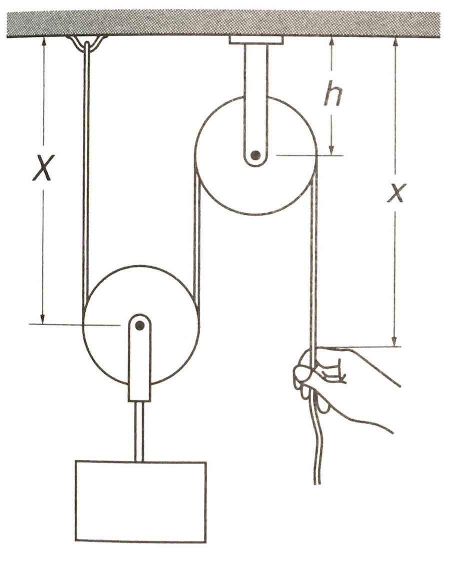
Fig. 7 Lifting a mass using a pulley system.

We work out the acceleration \(\ddot{x}\) of the hand, which is of course related to the force with which the hand pulls (\(F_h = m\ddot{x}\)), and compare it to the acceleration of the block \(\ddot{X}\). Assuming that the length of the string is a constant \(l\) and the radius of the wheels is \(R\), we know that

(17)\[\begin{align}\nonumber l = X + \pi R + (X-h) + \pi R + (x-h)\, . \end{align}\]

Rearranging this, we obtain a relation between \(x\) and \(X\):

(18)\[\begin{align}\nonumber x = l - 2(X+\pi R - h)\, . \end{align}\]

Taking the second derivative to obtain the relationship between the accelerations of the hand and the mass, we find

(19)\[\begin{align}\nonumber \ddot{X} = -\frac12 \ddot{x}\, . \end{align}\]

To raise the block a distance \(s\), the hand must pull down the rope twice that distance downwards. Note the relative signs and the direction of pulling and lifting. To work out the force with which the hand must pull, we can use the work done on the block:

(20)\[\begin{align}\nonumber W = F s = mgs\, . \end{align}\]

By conservation of energy, the work done by the hand is equal to the work done on the block, and we find

(21)\[\begin{align}\nonumber W_h = F_h \times 2s = mgs \qquad\Rightarrow\qquad F_h = \frac12 mg\, . \end{align}\]

In other words, we have to apply only half the force that we would need if we were to lift the block directly, but the trade-off is that we need to pull the rope twice the distance we want to move the block. Using more pulleys you can lift heavier objects with the same force.

---

Terminal velocity

We want to calculate the terminal velocity of a sphere with mass \(m\) in a fluid under gravity. We can start with the exercise in problem set 2, where we looked at the drag force. Here, we have a drag force against the direction of the velocity \(v\):

(22)\[\begin{align} F_{\rm drag} = -bv\, , \end{align}\]

as well as the gravitational force \(F_{\rm gr} = mg\) due to the gravitational acceleration \(g\). The net force experienced by the sphere is the sum of these two forces,

(23)\[\begin{align} F_{\rm net} = F_{\rm gr} + F_{\rm drag} = mg - bv\, . \end{align}\]

The positive direction is chosen downwards. We set this equal to \(F_{\rm net} = ma\), but instead of finding the position \(x(t)\), we want to find a differential equation for the velocity \(v(t)\), since we are interested in the terminal velocity. That is actually easier:

(24)\[ \frac{\d v}{\d t} = -\frac{b}{m}v + g\, .\]

To solve a differential equation, we often make a so-called Ansatz (German for `guess’). Here, we will try

(25)\[\begin{align} v(t) = u + w \e^{-st}\, , \end{align}\]

where we need to find \(u\), \(w\) and \(s\). First we calculate \(\dot{v}(t)\):

(26)\[\begin{align} \frac{\d v}{\d t} = -ws\, \e^{-st}\, , \end{align}\]

and we substitute this back into the differential equation (24):

(27)\[\begin{align} -ws\, \e^{-st} = -\frac{b}{m}\left( u + w \e^{-st} \right) + g\, . \end{align}\]

This can only be a valid equation if the factors in front of the exponentials are the same, and the remaining constants sum to zero:

(28)\[\begin{align} -ws = -\frac{b}{m}w \qquad\text{and}\qquad -\frac{b}{m} u + g = 0\, . \end{align}\]

From this we find that

(29)\[\begin{align} s = \frac{b}{m} \qquad\text{and}\qquad u = \frac{mg}{b}\, . \end{align}\]

We do not know what \(w\) is yet. To find it, we need to use the initial condition for the differential equation, e.g., \(v(t=0) = v_0\). The we find

(30)\[\begin{align} v(t) = \frac{mg}{b} + w\, \e^{-bt/m}\, . \end{align}\]

Hence

(31)\[\begin{align} v(0) = \frac{mg}{b} + w\, \e^0 = v_0 \qquad\to\qquad w = v_0 - \frac{mg}{b}\, . \end{align}\]

This leads to the final result

(32)\[\begin{align} v(t) = \frac{mg}{b} \left( 1 - \e^{-bt/m}\right) +v_0\, \e^{-bt/m}\, . \end{align}\]

When \(g=0\) we recover the result from problem set 2, as required. But more interestingly, we can find the terminal velocity by taking the limit of \(t\to\infty\). The exponetials will tend to zero in this limit, so we have

(33)\[\begin{align} v_{\rm terminal} = \lim_{t\to\infty} v(t) = \frac{mg}{b}\, . \end{align}\]

This is independent of the initial velocity \(v_0\), but it does depend on \(b\), which itself captures all the relevant information about the shape and density of the object, as well as the viscosity of the fluid or gas.