\(\renewcommand{\a}{\mathbf{a}}\) \(\renewcommand{\b}{\mathbf{b}}\) \(\renewcommand{\c}{\mathbf{c}}\) \(\newcommand{\g}{\mathbf{g}}\) \(\newcommand{\x}{\mathbf{x}}\) \(\newcommand{\y}{\mathbf{y}}\) \(\newcommand{\z}{\mathbf{z}}\) \(\renewcommand{\r}{\mathbf{r}}\) \(\renewcommand{\v}{\mathbf{v}}\) \(\renewcommand{\u}{\mathbf{u}}\) \(\newcommand{\kk}{\mathbf{k}}\) \(\newcommand{\p}{\mathbf{p}}\) \(\newcommand{\m}{\mathbf{m}}\) \(\renewcommand{\d}{\mathrm{d}}\) \(\newcommand{\e}{\mathrm{e}}\) \(\newcommand{\A}{\mathbf{A}}\) \(\newcommand{\B}{\mathbf{B}}\) \(\newcommand{\D}{\mathbf{D}}\) \(\newcommand{\E}{\mathbf{E}}\) \(\newcommand{\J}{\mathbf{J}}\) \(\newcommand{\F}{\mathbf{F}}\) \(\newcommand{\M}{\mathbf{M}}\) \(\renewcommand{\H}{\mathbf{H}}\) \(\renewcommand{\P}{\mathbf{P}}\) \(\newcommand{\R}{\mathbf{R}}\) \(\renewcommand{\l}{\mathbf{l}}\) \(\renewcommand{\S}{\mathbf{S}}\) \(\newcommand{\V}{\mathbf{V}}\) \(\renewcommand{\L}{\mathbf{L}}\) \(\newcommand{\ms}{\;\text{m}\;\text{s}^{-1}}\) \(\newcommand{\mss}{\;\text{m}\;\text{s}^{-2}}\)

\(\DeclareMathOperator{\sinc}{sinc}\)

\(\newcommand{\kopje}[2]{\vskip0.5em\noindent\textbf{\textsf{{\color{OliveDrab}{Week #1}:}~ #2}}}\) \(\newcommand{\homework}[1]{\noindent{\color{FireBrick}{\textbf{\textsf{Homework:}}} #1}}\) \(\newcommand{\tutorial}[1]{\noindent{\color{SteelBlue}{\textbf{\textsf{Tutorial:}}} #1}}\) \(\newcommand{\problems}[1]{\noindent{\color{LightSlateGrey}{\textbf{\textsf{Weekly problems:}}} #1}}\)

\(\newcommand{\af}[1]{[A\&F: #1]}\) \(\newcommand{\basis}[1]{\hat{\text{e}}_{#1}}\)

Polar coordinates and circular motion

Polar coordinates

When an object moves in a circle in the \(xy\)-plane around the origin \(O\), the \(x\) and \(y\) coordinates as a function of time are given by

(34)\[ x(t) = a \cos\omega t \qquad\text{and}\qquad y(t) = a \sin\omega t\, ,\]

where in this case the object lies on the \(x\)-axis at time \(t=0\), and the radius of the circle is \(a\). The angular velocity of the particle is \(\omega\), to which we will return in a moment. The \(x\) and \(y\) coordinates are components of a two-dimensional vector

(35)\[\begin{align} \r(t) = \begin{pmatrix} x(t) \\ y(t) \end{pmatrix}\, , \end{align}\]

as we encountered before. While the Cartesian coordinates \(x\) and \(y\) (and \(z\) in three dimensions) are often very convenient, for circular motion there are other coordinates that are more convenient, namely polar coordinates \(r\) and \(\theta\). Here \(r\) is the distance to the origin, and \(\theta\) is the angle between the \(x\)-axis and the line from the origin to the object’s position. The reason these polar coordinates are more convenient is that for the circular motion above the distance to the origin stays constant (\(r=a\)), so we should be able to reduce the two-coordinate problem (\(x\) and \(y\)) to a single-coordinate problem (\(\theta\) only).

Fig. 8 Polar coordinates against a grid of Cartesian coordinates.

The relation between the Cartesian coordinates and the polar coordinates is given by

(36)\[ x = r \cos\theta \qquad\text{and}\qquad y = r \sin\theta\, .\]

Note that these are always true, and carry a completely different meaning than the expressions in equation (34), which look superficially similar. Equation (34) describes the motion of a particle over time, while equation (36) describes the relation between two coordinate systems.

We can invert equation (36) to get \(r\) and \(\theta\) in terms of \(x\) and \(y\):

(37)\[ r = \sqrt{x^2+y^2} \qquad\text{and}\qquad \theta = \arctan\left(\frac{y}{x}\right)\, .\]

This means that \(r\) runs from zero to infinity (we take the positive square root), and \(\theta\) runs from zero to \(2\pi\) (This is another difference between equation (34) and equation (36): the mapping between coordinate systems has to make sure the plane is covered exactly once by each coordinate system, whereas \(\omega t\) can take values much greater than \(2\pi\) as it describes the trajectory of a particle going around in circles indefinitely.):

(38)\[\begin{align} r \in [0,\infty) \qquad\text{and}\qquad \theta \in [0,2\pi)\, . \end{align}\]

We can write the motion of the object in equation (34) in terms of polar coordinates as

(39)\[ r(t) = a = \text{constant} \qquad\text{and}\qquad \theta(t) = \omega t\, .\]

This means, as noted before, that we have to worry only about \(\theta\) as a variable with respect to time. More general motion will again require two variables \(r\) and \(\theta\), or \(x\) and \(y\). As a rule of thumb, if the motion looks more like linear motion (but not quite), Cartesian coordinates may be better, and if it is closer to circular motion polar coordinates are likely better.

Returning to our example, we have to consider the basis vectors of our coordinate systems. For the Cartesian system this is simple:

(40)\[\begin{split} \r(t) = \begin{pmatrix} a\cos\omega t \\ a \sin\omega t \end{pmatrix} = a\cos\omega t \begin{pmatrix} 1 \\ 0 \end{pmatrix} + a\sin\omega t\begin{pmatrix} 0 \\ 1 \end{pmatrix} = a\cos\omega t\; \basis{x} + a\sin\omega t\; \basis{y}\, ,\end{split}\]

where we introduced the basis vectors

(41)\[\begin{align} \basis{x}= \begin{pmatrix} 1 \\ 0 \end{pmatrix} \qquad\text{and}\qquad \basis{y} = \begin{pmatrix} 0 \\ 1 \end{pmatrix} \, . \end{align}\]

Wherever we are in the \(xy\)-plane, the basis vector \(\basis{x}\) always points in the direction of the positive \(x\)-axis, and the basis vector \(\basis{y}\) always points in the direction of the positive \(y\)-axis. However, the basis vectors \(\basis{r}\) and \(\basis{\theta}\) point in different directions at different locations in the plane. The vector \(\basis{r}\) always points away from the origin, while \(\basis{\theta}\) is orthogonal to \(\basis{r}\) and lies tangential to the circle centred around the origin and intersecting the point \((r,\theta)\). It points in the counter-clockwise direction.

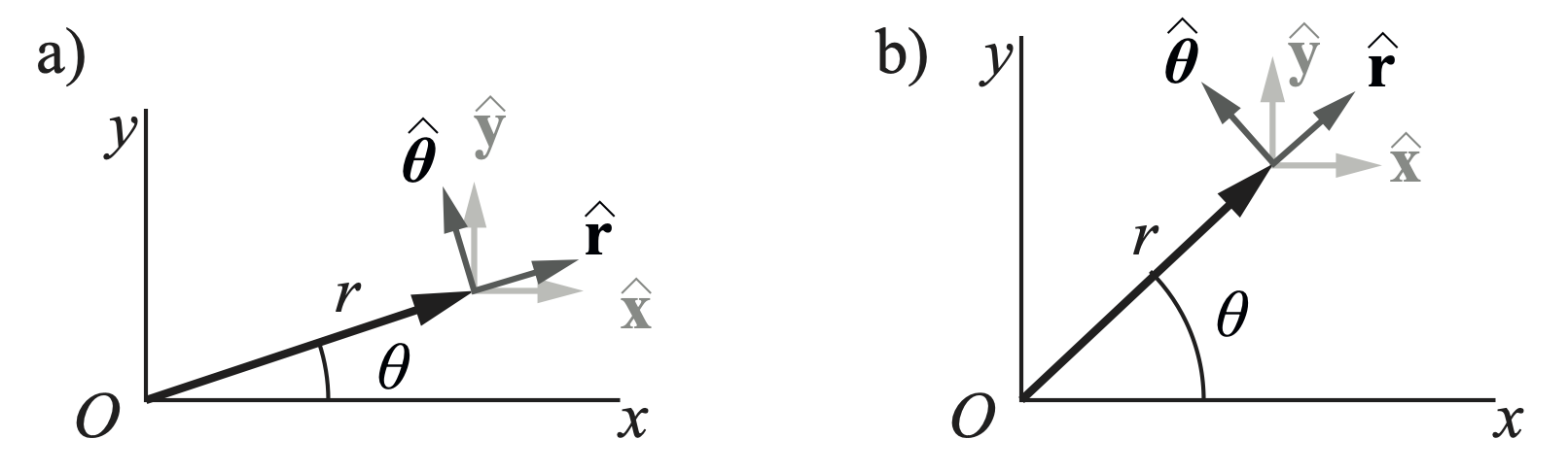
Fig. 9 Changing basis vectors in polar coordinates.

If you want to know the basis vectors \(\basis{r}\) and \(\basis{\theta}\) in terms of \(\basis{x}\) and \(\basis{y}\), you have to use trigonometry. You can readily infer from figure 10 that this gives

(42)\[ \basis{r} = \cos\theta\; \basis{x} + \sin\theta\; \basis{y} \qquad\text{and}\qquad \basis{\theta} = -\sin\theta\; \basis{x} + \cos\theta\; \basis{y}\, .\]

We will use these relations a lot in what follows. The changing directions of \(\basis{r}\) and \(\basis{\theta}\) become particularly important when we take derivatives, for example when we want to work out the velocity and acceleration of an object. We will show how this works in a moment. First, what does a vector \(\r\) look like in polar coordinates? It is remarkably compact:

(43)\[ \r = r\, \basis{r} = a\, \basis{r}\, ,\]

where the second equality is specifically for our example. You should convince yourself by drawing \(\r\) and \(\basis{r}\) that there is no \(\basis{\theta}\) contribution in the expression of the general vector \(\r\) in polar coordinates.

Circular motion and the Cross Product

For uniform rotations in three dimensions, where the angular velocity \(\omega\) is constant, there is another convenient and often-used description of circular motion that involves the cross product. The cross product between two vectors \(\a\) and \(\b\) is written as

(44)\[\begin{align} \a\times\b = (a_y b_z - a_z b_y) \basis{x} + (a_z b_x - a_x b_z) \basis{y} + (a_x b_y - a_y b_x) \hat{\z}\, . \end{align}\]

This can be written as

(45)\[\begin{align} \a\times\b = ab\sin\theta \, \hat{e}_N\, , \end{align}\]

where \(\theta\) is the angle between \(\a\) and \(\b\), and \(\hat{e}_N\) is the vector normal to the plane spanned by \(\a\) and \(\b\). This plane has an orientation: if the fingers on your right hand point in the direction as you rotate the vector \(\a\) to vector \(\b\), your thumb will point in the direction of \(\hat{e}_N\).

Define the angular velocity \(\omega\) as

(46)\[\begin{align} \omega = \frac{\d \theta}{\d t}\, , \end{align}\]

as before. The speed along a circle with radius \(R\) is then

(47)\[\begin{align} v = \omega R\, . \end{align}\]

However, in three dimensions not all possible points lie in the \(xy\)-plane, and we want a relation between \(\v\), \(\r\), and \(\omega\). To this end we orient \(\omega\) along the \(z\)-axis, so we can write \(\vec{\omega} = \omega \hat{\z}\), and we pick a point \(A\) along a circle with radius \(R\) above the \(xy\)-plane. The position vector pointing to \(A\) is \(\r\). This is shown in Fig. 11.

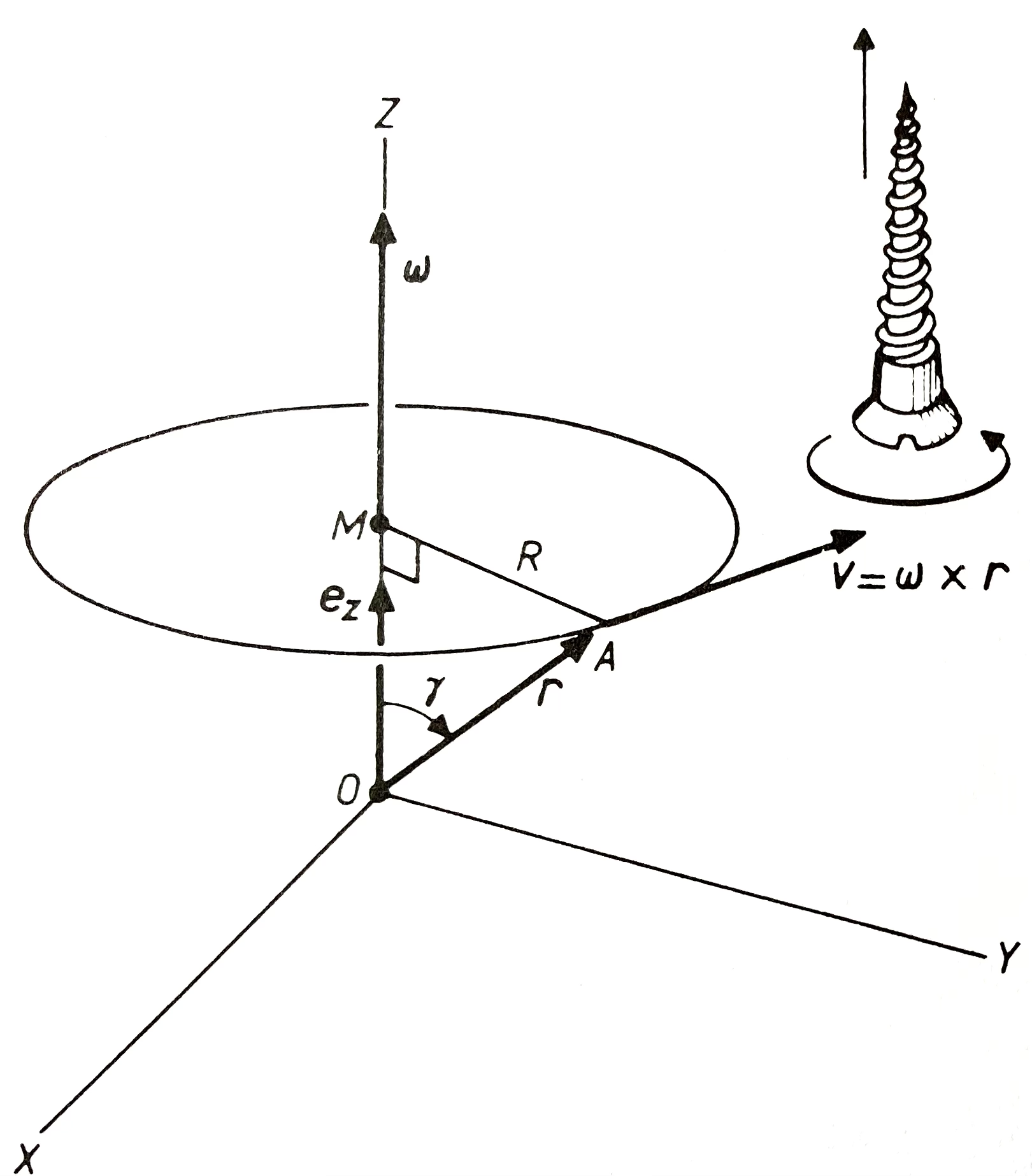
Fig. 10 Vector relation between (constant) angular velocity \(\vec{\omega}\), linear velocity \(\v\) and position \(\r\).

From the figure, \(R = r\sin\gamma\), with \(\gamma\) the angle between the vector \(\hat{\z}\) and \(\r\). Hence, the linear speed around the circle is

(48)\[\begin{align} v = \omega r \sin\gamma\, . \end{align}\]

However, this can be written as a cross product between \(\vec{\omega}\) and \(\r\):

(49)\[\begin{align}%\label{eq:njbgtuehoi4wrnd} \v = \vec{\omega}\times\r\, . \end{align}\]

This is true only for circular motion with constant \(r\) and \(\gamma\). While this is neat and compact, it is not so clear yet why this is a nice form. However, it allows us to treat the time derivative \(\d/\d t\) in the case of constant circular motion as the cross product with the angular velocity: \(\vec{\omega}\times\cdot\). We can find the acceleration from the time derivative of \(\v\), and therefore for circular motion with constant \(\omega\) we obtain

(50)\[\begin{align} \a = \frac{\d\v}{\d t} = \frac{\d}{\d t} \vec{\omega}\times\r = \vec{\omega}\times \frac{\d\r}{\d t} = \vec{\omega}\times\v\, . \end{align}\]

In its most useful form, we have

(51)\[\begin{align}%\label{eq:nfvjrowu32wireh} \a = \vec{\omega}\times(\vec{\omega}\times\r)\, . \end{align}\]

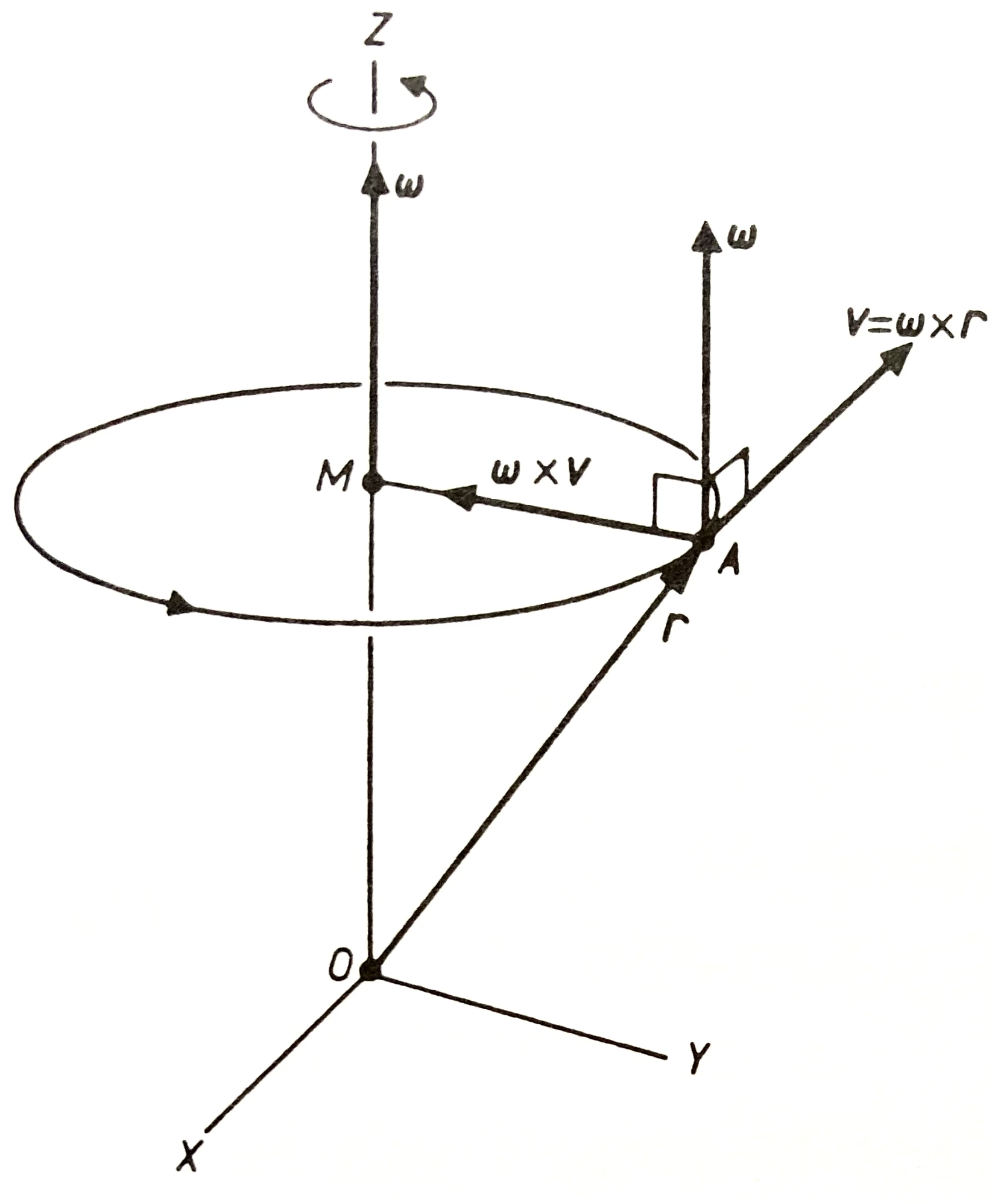
Fig. 11 Acceleration towards the centre \(M\).

Torque described as a vector

As we have seen, the momentum \(\p\) of a body with mass \(m\) is the amount of linear motion of the body. To change this amount of linear motion, we need to apply a force \(\F = \d\p/\d t\). The situation changes somewhat when we consider rotational motion. We cannot merely apply a force to set a body in rotational motion, we need a moment, or torque \(\bm{\tau}\). You are already familiar with torque: a lever or see-saw has two forces (e.g., gravity at the end of the see-saw and the normal force at the fulcrum), in opposite direction and with a distance \(d\) apart. You have been writing this as \(\tau = Fd\). Now we will give this expression its proper vector form[1].

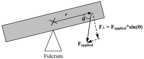
Fig. 12 Figure: Torque as a combination of vectors \(\r\) and \(\F_{\rm applied}\).

Consider the see-saw. Let \(\F\) be the force down on the tip of the see-saw, and let \(\r\) be the distance vector from the fulcrum to the top of the see-saw where the force \(\F\) is applied. This will create a torque \(\bm{\tau}\) that points in the direction of the angular velocity \(\bm{\omega}\). All these vectors are perpendicular, so we must use the cross product to relate them. When we work out the directions (do this!) we find

\[ \bm{\tau} = \r\times \F = \r\times \frac{\d\p}{\d t}\, . \]

---

Example:
Let’s return to the example of the ladder leaning against a wall, as introduced in section 4. You were asked to draw the forces on the ladder. Referring back to the forces you drew, identify two torques on the ladder. Given static friction \(\mu\) with the floor only, calculate (i.e., find an expression for) the shallowest angle of the ladder with the floor for which the ladder is at rest. You will need to define all the relevant quantities (mass, etc.).

---

Spherical and cylindrical coordinates

In three dimensions, there are two main sets of coordinates associated with rotational motion: cylindrical and spherical. Their names give you a clue when you want to use what. These coordinate systems will be discussed in detail in the rest of your degree, so here we only give their relation to the Cartesian coordinates.

Cylindrical coordinates are very much like polar coordinates, but supplemented with a “Cartesian” third dimension, \(z\). Instead of \(r\) as the distance to the origin, we typically use \(\rho\) and \(\phi\). Do not confuse \(\rho\) with a density!

(52)\[\begin{align} x & = \rho \cos\phi \cr y & = \rho \sin\phi \cr z & = z\, . \end{align}\]

The last one feels a bit redundant, but it reminds us that there is a third dimension. You should work out \(\rho\) and \(\phi\) in terms of \(x\), \(y\), and \(z\).

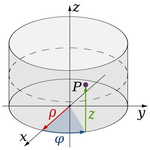
Fig. 13 Cylindrical coordinates

Spherical coordinates are often the coordinates of choice when the potential depends only on \(r\), the distance to the origin. They are defined by the relations

(53)\[\begin{align} x & = r \cos\phi\sin\theta \cr y & = r \sin\phi\sin\theta \cr z & = r\cos\theta\, . \end{align}\]

You should construct the inverse relation, specifying \(r\), \(\theta\), and \(\phi\) in terms of \(x\), \(y\), and \(z\).

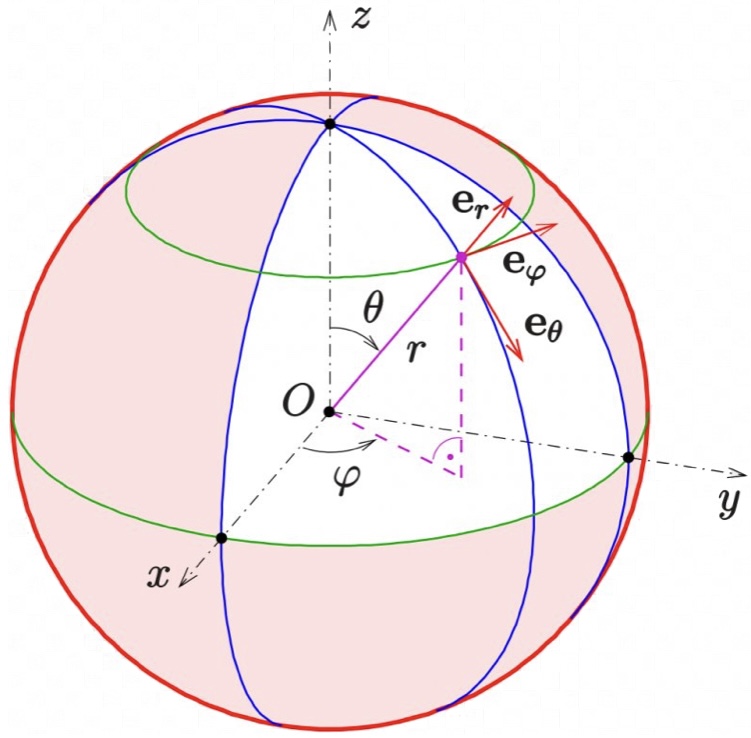
Fig. 14 Spherical coordinates.

---

[1]

Not least because in this form \(Fd\) could be mistaken for work.