4. Functions and graphs#
After studying this section, you should
be able to find the domain and the range of a function;
be able to draw graphs of functions;
be able to compose functions;
understand the difference between composition of functions and (point-wise) multiplication of functions;
understand and be able to find inverse functions;
understand the trigonometric functions and draw their graphs.
4.1. Functions, Rules and Domains#
Loosely speaking, a function is something which takes an input (often a number) and gives an output (often another number). A function \(f\) must have a domain, a rule and a codomain.
The domain tells us which things (or values) the function takes as an input.
The rule tells us how to work out the output of the function. Note that the rule will always give just one output for each input.
The codomain tells us what the function might give as an output.
In the examples we will look at, the domain of the function will always be a set of numbers of some kind and the codomain is likely to be \(\mathbb{R}\) (that is, the function will give out real numbers).
A function is stated fully by giving each of the domain, the rule and the codomain. To denote a function with domain \(D\), codomain \(C\) and rule \(f(x)\) we write \(f:D\rightarrow C,\) \(x\mapsto f(x)\). For example, we may have a function that takes in real numbers and gives out real numbers according to the rule \(f(x)=x^2\); we would write this as
or
The codomain is the least important of the three properties of the function and often it is obvious what the codomain should be (usually \(\mathbb{R}\)). So we may sometimes omit it and just write things like
“\(f\) has domain \(\{x\in\mathbb{R}~:~ -1\leq x\leq 1\}\) and is defined by \(f(x)=x^2\)”.
Example 4.1
(i) Let \(f\) have rule \(f(x) = x^2\) and domain \(\{ x \in \mathbb{R}:-1 < x < 1\}\). Then \(x = 0\) is in the domain and we have \(f(0) = 0^2 = 0\). On the other hand, \(x = 2\) and \(x=1\) are not in the domain, so \(f(2)\) and \(f(1)\) are undefined.
(ii) Let \(g\) have rule \(g(x) = \sqrt{x}\) and domain \(\{x \in\mathbb{R}\::\: x \geq 0\}\). Then \(x = 9\) is in the domain, and \(g(9) = 3\). Also \(x = \frac 52\) is in the domain and \(g(\frac 52) = \sqrt{\frac 52}\).
(iii) Let \(h\) have rule \(h(x) = \frac 1x\) and domain \(\{ x \in\mathbb{R}\::\: x \neq 0\}\). Then \(x = 3\) is in the domain and \(h(3) = \frac 13\). Also \(x = -\frac 72\) is in the domain and \(h(-\frac 72) = \frac{\phantom{aa}1\phantom{aa}}{-\frac 72} = - \frac 27\).
Note
Examples (ii) and (iii) above are the most common examples of functions, where the domain is all the \(x\) for which the rule is defined; that is, all the \(x\) which make sense in the rule.
In (ii), \(\sqrt{x}\) requires \(x \geq 0\).
In (iii), \(\frac 1x\) requires \(x \neq 0\).
However we can have examples like (i) where the domain is only some of the \(x\) for which the rule is defined. In this example, \(x^2\) is defined for all \(x\) but there may be some other reason why we restrict to \(-1 < x < 1\) (for example, we may have a practical situation where there is a physical constraint on \(x\) limiting it to \(-1 < x < 1\)).
Example 4.2
The function \(f\) has rule \(f(x) = \frac {\sqrt{x}}{x-1}\) and the domain of \(f\) is all the \(x\) for which \(\frac {\sqrt{x}}{x-1}\) is defined. Find the domain of \(f\) and suggest a suitable codomain.
Solution.
Similarly to above, \(\sqrt{x}\) is defined for \(x \geq 0\) and \(\frac{1}{x-1}\) is defined for \(x \neq 1\). So the domain of \(f\) is \(\{ x:x \geq 0 \mbox{ and } x\neq 1\}\). As usual, a suitable codomain here is \(\mathbb{R}\).

Fig. 4.1 Domain of \(f\)#
Note
If a function has no restriction on \(x\) then the domain will be \(\mathbb{R}\), the complete set of real numbers. For example, the function \(f\) with rule \(f(x) = x + 3\) could have domain \(\mathbb{R}\).
Exercise
Each part below refers to a function \(f\). In each part the domain is all the values of \(x\) for which the expression for \(f(x)\) is defined. Find the domain of each function.
(i) \(f(x) = \sqrt{3-x}\);
(ii) \(f(x) = \frac{1}{2-x}\);
(iii) \(f(x) = \sqrt{x+2}+ \frac{1}{x-3}\);
(iv) \(f(x) = \sqrt{(x-1)(x-3)}\);
(v) \(f(x) = \frac{\sqrt{2-x}}{(x+5)(x+7)}\).
Solution
(i) \(f(x)=\sqrt{3-x}\) is defined whenever \(3 - x \geq 0,\) that is when \(x \leq 3\). So the domain of \(f\) is \(\{ x\in\mathbb{R}\::\: x \leq 3\}\).
.png)
Fig. 4.2 Domain of \(\sqrt{3-x}\)#
(ii) \(f(x)=\frac 1{2-x}\) is defined whenever \(2-x \neq 0,\) that is when \(x \neq 2\). So the domain of \(f\) is \(\{x\in\mathbb{R}\::\: x \neq 2\}\).
.png)
Fig. 4.3 Domain of \(\frac{1}{2-x}\)#
(iii) \(f(x)=\sqrt{x+2}\) is defined whenever \(x+2 \geq 0,\) that is when \(x \geq -2\). And \(\frac 1{x-3}\) is defined whenever \(x-3 \neq 0,\) that is when \(x \neq 3\). So the domain of \(f\) is \(\{x\in\mathbb{R}\::\: x \geq -2 \mbox{ and } x \neq 3\}\).
+1,(x-3).png)
Fig. 4.4 Domain of \(\sqrt{x+2}+\frac{1}{x-3}\)#
(iv) \(\sqrt{(x-1)(x-3)}\) is defined whenever \((x-1)(x-3) \geq 0,\) that is when \(x-1>0\) and \(x-3>0\) or when \(x-1<0\) and \(x-3<0\). In the first case, we get that \(x \geq 1\) and \(x \geq 3\) (so that \(x\geq3\)), and in the second case we get that \(x \leq 1\) and \(x \leq 3\) (so that \(x\leq1\)). So the domain is \(\{x\in\mathbb{R}\::\: x \leq 1 \mbox{ or }x \geq 3\}\).
(x-3)).png)
Fig. 4.5 Domain of \(\sqrt{(x-1)(x-3)}\)#
(v) \(\sqrt{2-x}\) is defined whenever \(2-x \geq 0,\) that is when \(x\leq 2\). And \(\frac{1}{(x+5)(x+7)}\) is defined whenever \(x+5 \neq 0\) and \(x+7 \neq 0,\) that is when \(x \neq -5\) and \(x \neq -7\). So the domain of \(f\) is \(\{x\in\mathbb{R}:x \leq 2 \mbox{ and } x \neq -5 \mbox{ and } x \neq -7\}\). \
,((x+5)(x+7)).png)
Fig. 4.6 Domain of \(\frac{\sqrt{2-x}}{(x+5)(x+7)}\)#
Convention: If we are given a function \(f\) and are only told the rule, then we should assume that the domain is all \(x\) for which the expression is defined.
Exercise
Find the domain of the functions of
(i) \(f(x) =\displaystyle \frac 1{x-3}\);
(ii) \(f(x) = \displaystyle \sqrt{10-x}\);
(iii) \(f(x) = \displaystyle \sqrt{25 -x^2}\);
(iv) \(f(x) = \displaystyle \frac 1{25-x^2}\);
(v) \(f(x) = \displaystyle \frac 1{25 +x^2}\).
4.2. Graphs of Functions#
4.2.1. Introduction#
Given a function \(f\) with domain being some subset of the real numbers and codomain \(\mathbb{R}\) we can create a graph where \(y=f(x)\). As before, we can get a feel for the graph by taking some values of \(x\) in the domain and plotting the points \((x,f(x))\).
Example 4.3
The graph of \(f(x) = x^2\) where the domain is \(\{x\in\mathbb{R}~: -1 < x < 1\}\).
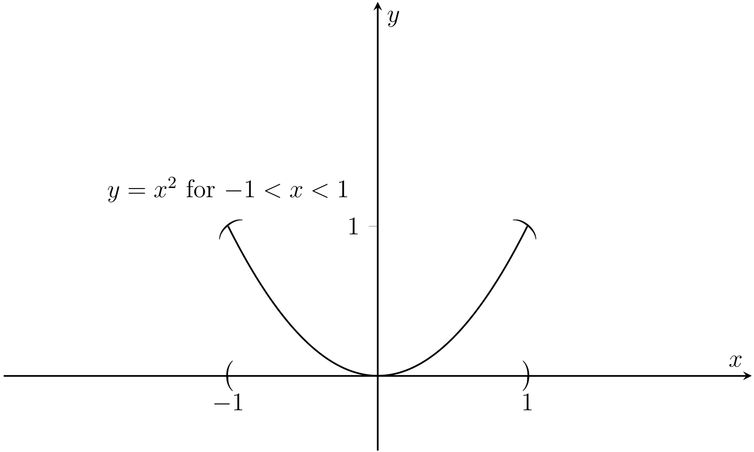
Fig. 4.7 Graph of \(f(x)=x^2\) with domain \(\{x\in\mathbb{R}~: -1 < x < 1\}\).#
The graph of \(f(x) = \frac 1x\) where the domain is \(\{ x\in\mathbb{R}:x \neq 0 \mbox{ and } - 3 \leq x \leq 3\}\).
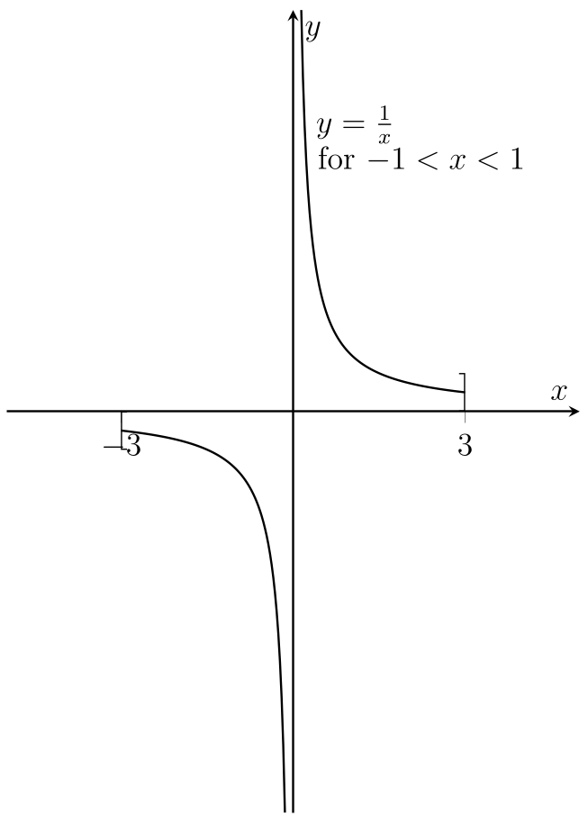
Fig. 4.8 \(y=\frac{1}{x}\) for \(x\neq 0\) and \(-3\leq x\leq 3\).#
Note: Remember that a plot is obtained by putting a couple of points \((x, f(x))\) into the coordinate axes and then connecting them with a smooth curve, while a sketch is obtained by using mathematical insight.
Note that by now you should be able to sketch the graphs of linear functions, that is the graph of a function of the form \(y = ax +b\) where \(a \neq 0\). These are straight line graphs with gradient \(a\) and \(y\)-intercept \(b\). If you have problems with this, have a look at \href{https://www.sheffield.ac.uk/media/30732/download?attachment}{this resource} (clicking will download a pdf file).
4.2.2. Sketching graphs of functions#
Example 4.4
Sketch the graph of \(f(x) = x^2\) with domain \(\{ x:-2 \leq x < 3\}\).
Solution.
We sketch the graph of \(y = x^2\), noting that we only allow \(x\) to vary between \(-2\) and \(3\). We also mark on the graph that \(-2\) is included, whilst \(3\) is not.
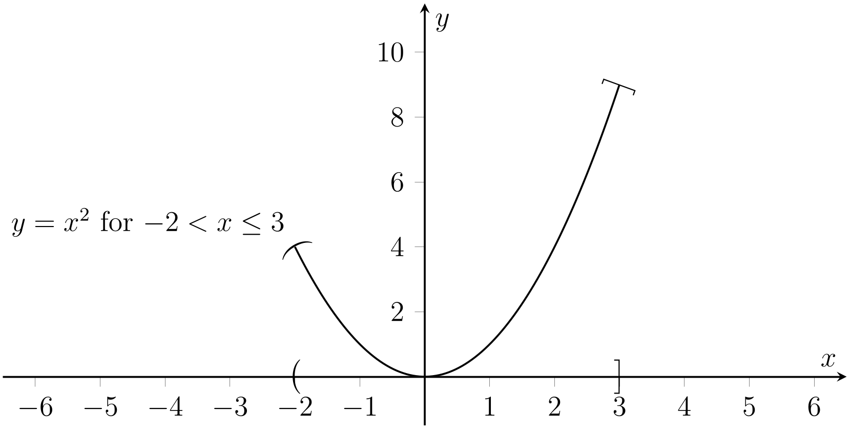
Fig. 4.9 Graph of the function \(f(x) = x^2\) with domain \(\{ x:-2 \leq x < 3\}\).#
Exercise
Sketch the graphs of the following functions \(f\):
(i) \(f(x) = 2x -3\) where the domain is \(\{ x\in\mathbb{R}\::\: 1 \leq x \leq 4\}\).
(ii) \(f(x) = x^2 -2x -3\) where the domain is \(\{ x\in\mathbb{R}\::\: -2 < x \leq 2\}\).
Solution
(i) Let \(f(x)=2x-3\) with domain \(\{ x\in\mathbb{R}\::\: 1 \leq x \leq 4\}\). We sketch \(y = 2x -3\). When \(x = 0\), \(y = -3,\) and when \(y=0\) when \(2x-3=0\), that is \(x=\frac{3}{2}\). Note that at \(x=1\), \(y=-1\) and at \(x=4\), \(y=5\).
We only draw the graph between \(x=1\) and \(x=4\).
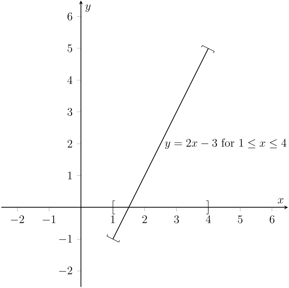
Fig. 4.10 Graph of \(f(x)=2x-3\) with domain \(\{ x\in\mathbb{R}\::\: 1 \leq x \leq 4\}\).#
(ii) Let \(f(x) = x^2 -2x -3\) with domain \(\{ x\in\mathbb{R}\::\: -2 < x \leq 2\}\).
We complete the square to get \(f(x) = (x -1)^2 - 1-3 = (x-1)^2 - 4\). Thus \(f(x)\) has a minimum at \(x=1\) and \(y=-4\). When \(x=0\), \(y=-3\) and \(y=0\) where \(x=1\pm 2=-1\) or \(3\).
We only draw the graph between \(x=-2\) and \(x=2\).
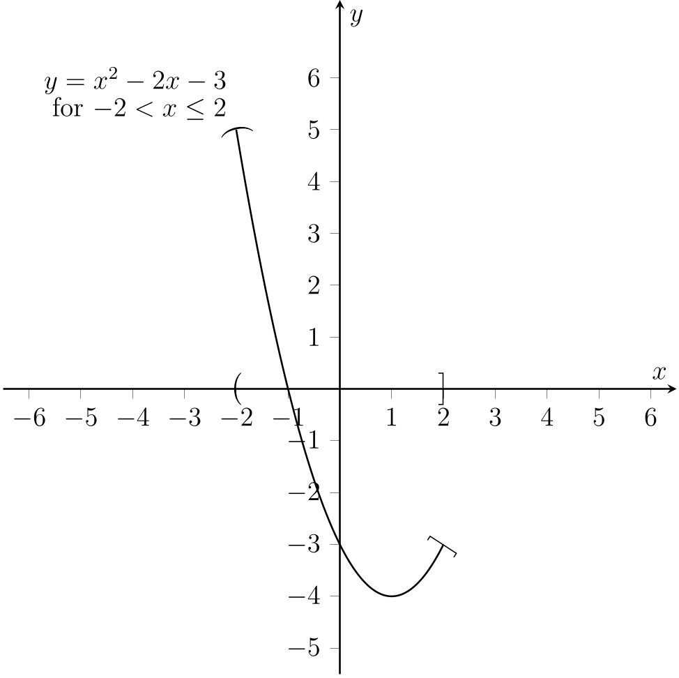
Fig. 4.11 Graph of \(f(x) = x^2 -2x -3\) with domain \(\{ x\in\mathbb{R}\::\: -2 < x \leq 2\}\).#
4.3. The Range of a Function#
Definition 4.1 (Range of a function)
The range of a function \(f\) is the precise set of values that \(f(x)\) gives as outputs as \(x\) varies over the domain. It is a subset of the codomain.
If \(f\) is a function of real numbers and we have drawn a graph of \(y=f(x)\) then the range can be found as the set of points on the \(y\)-axis which are horizontally in line with the graph.
Example 4.5
The function \(f\) has \(f(x) = 2x -3\) and domain \(\{ x\in\mathbb{R}:1 \leq x \leq 4\}\). Find the range of \(f\).
Solution.
We sketch the graph of \(f\). Note we did this in Fig. 4.10.
Fig. 4.12 Graph of the function \(f(x) = 2x -3\) with domain \(\{ x\in\mathbb{R}:1 \leq x \leq 4\}\).#
So the range of \(f\) is the \(\{ y\in\mathbb{R}\::\: -1 \leq y \leq 5\}\).
Exercise
The function \(f\) has \(f(x) = x^2 -2x -3\) and domain \(\{ x\in\mathbb{R}:-2 < x \leq 2\}\). Find the range of \(f\).
Exercise
The function \(f\) has \(f(x) = \frac 1x\) and domain \(\{ x \in\mathbb{R}\::\: x \geq 2\}\). Find the range of \(f\).
Solution
We sketch the graph of \(y = \frac 1x\). Note that we don’t really need to restrict the graph to our given domain as we can read up our range from the full graph as long as we remember the restriction.
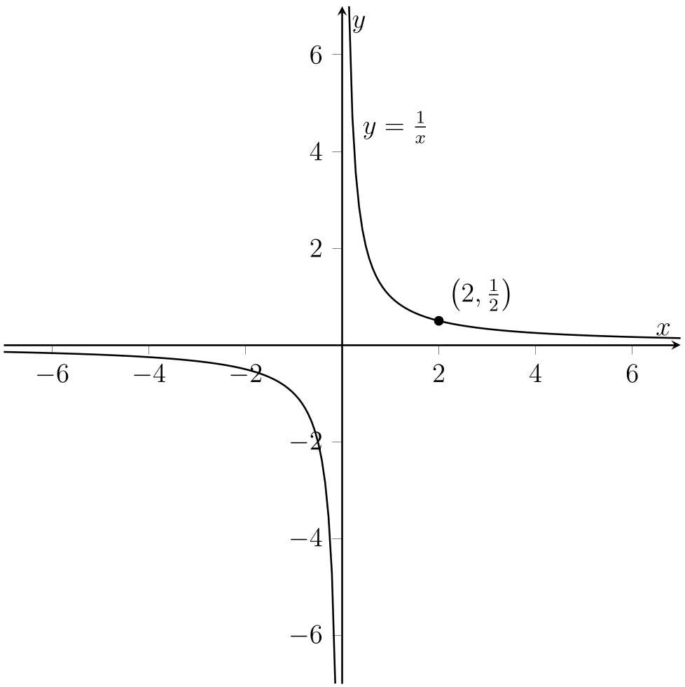
Fig. 4.14 Graph of the function \(y=\frac{1}{x}\) with the point \((2,\frac{1}{2})\) marked.#
Remembering that the domain of \(f\) is \(\{ x \in\mathbb{R}\::\: x \geq 2\}\) we see that the range of \(f\) is \(\{ y\in\mathbb{R}:0< y \leq \frac 12\}\).
4.4. Composition of Functions#
Often we find we can compose two functions by substituting one into another.
Example 4.6
Let \(f(x) = 2x\) and \(g(x) = x +3\). Find
(i) \(f(g(x))\)
(ii) \(g(f(x))\).
Solution.
(i) To find \(f(g(x))\) we replace each occurrence of \(x\) in \(f(x)=2x\) by the expression for \(g(x)\), namely \(x+3\). Thus we get
Note that the brackets here are crucial!
(ii) Similarly to above, we must replace every occurrence of \(x\) in \(g(x)=x+3\) with the expression \(2x\). Thus
The above process is called composition of functions.
Exercise
Find \(f(g(x))\) and \(g(f(x))\) in each part below.
(i) \(f(x) = x^2,\) \quad \(g(x) = x-2\).
(ii) \(f(x) = \frac 1x,\) \quad \(g(x) = x^2 +3x\).
Solution.
(i) \(f(g(x)) = f(x-2) = (x-2)^2\) and \(g(f(x)) = g(x^2) = (x^2) -2 = x^2-2\).
(ii) \(f(g(x)) = f(x^2 +3x) = \frac{1}{x^2 +3x}\) and \(g(f(x)) = g(\frac 1x) = (\frac 1x)^2 + 3 \times (\frac 1x) = \frac 1{x^2} + \frac 3x\).
Exercise
Find (non-trivial) functions \(f\) and \(g\) such that
(i) \(f(g(x)) = \sqrt{x^2 +1},\)
(ii) \(f(g(x)) = (2x+3)^3,\)
(iii) \(f(g(x)) = \frac 1{x^2 +4}\).
Solution
The obvious possibilities are
(i) \(f(x) = \sqrt{x}\) and \(g(x) = x^2 +1\).
(ii) \(f(x) = x^3\) and \(g(x) = 2x +3\).
(iii) \(f(x) = \frac 1x\) and \(g(x) = x^2 +4\).
Note that we have point-wise multiplication of functions as we did with polynomials. That is, we can find \(f(x)\times g(x) - f(x)g(x)\). For example, if \(f(x) = x^2\) and \(g(x) = x+1\) then \(f(x)\times g(x) = f(x)g(x) = (x^2)(x+1) = x^3 +x^2\). This is not to be confused with the composition of the two functions. Especially in Semester 2, you will need to spot whether you have a composition of functions or a multiplication of functions.
Example 4.7
In each of the following, state if you deal with composition of functions, a product of functions, a division of function, a combination of these or nothing of that type:
(i) \(y_1 = \frac {x}{\sin x}\);
(ii) \(y_2 = \sin (x^2)\);
(iii) \(y_3 = x^{2} + x^3\);
(iv) \(y_4 = (x+2)(x+3)^2\);
(v) \(y_5 = x+ 3\);
(vi) \(y_6 = (x+3)^\frac 12\);
(vii) \(y_7 = \frac{x^2}{3}\);
(viii) \(y_8 = (x^2(x^3+5))^7\).
Solution.
(i) We have that \(y_1\) is a quotient of the two functions \(x\) and \(\sin x\)
(ii) \(y_2\) composes \(x^2\) as the “inner” function with the “outer” function \(\sin x\).
(iii) \(y_3\) is just adding up two standard functions
(iv) \(y_4\) is a product of the two functions \((x+2)\) and \((x+3)^2\) where \((x+3)^2\) is a “function of a function” with the inner function being \(x+3\) and the outer one \(x^2\).
(v) \(y_5\) is nothing exciting, just add two standard functions.
(vi) \(y_6\) is a composition of the functions \(x^\frac 12\) and \(x+3\).
(vii) \(y_7\) is the standard quadratic squashed by a factor of \(\frac 13\) in the \(y\)-axis.
(viii) Lastly, \(y_8\) is first of all a function of a function, namely \(x^7\) as the outer function and \(x^2(x^3+5)\) as the inner function, but the inner function is a product of the two functions \(x^2\) and \(x^3 +5\).
4.5. Inverse Functions#
Often, when given a function \(f\), we are given a value of \(x\) and asked to evaluate \(f(x)\). If we know the rule for \(f\), this is easy. However, sometimes we may be asked the reverse question: suppose \(f(x)=y\) for some \(y\). What is \(x\)? To do this, we need to find the inverse function, that is a function \(f^{-1}\) such that
Example 4.8
The function \(f\) is given by \(f(x) = \frac{3x-1}{x+2}\) for \(x\neq -2\). Suppose \(f(x)=y\). Find \(x\) in terms of \(y\).
Solution.
We approach this by making \(x\) the subject of the equation \(f(x)=y\). Now, for \(x\neq -2\),
So we have found that \(x = \frac{1+2y}{3-y}\) for \(y\neq 3\).
In fact what we have found here is precisely the inverse function, \(f^{-1}\). That is, we have found that
Note that we normally write functions in terms of the variable \(x\), so we would normally write
4.5.1. The geometrical connection between \(f\) and \(f^{-1}\)#
We hope to get a better understanding of how inverse functions work by looking at graphs of \(f\) and \(f^{-1}\) for various functions \(f\).
Example 4.9
Find \(f^{-1}\) when \(f(x) = 2x -3\). Sketch the graphs of \(y=f(x)\) and \(y=f^{-1}\) and spot a relation between them.
Solution.
Let \(y = 2x -3\) and solve for \(x\). We have
Hence \(\displaystyle f^{-1}(x) = \frac{x+3}{2}\). We sketch \(y = 2x -3\) and \(y = \frac {x+3}{2} = \frac 12 x + \frac 32\) below.
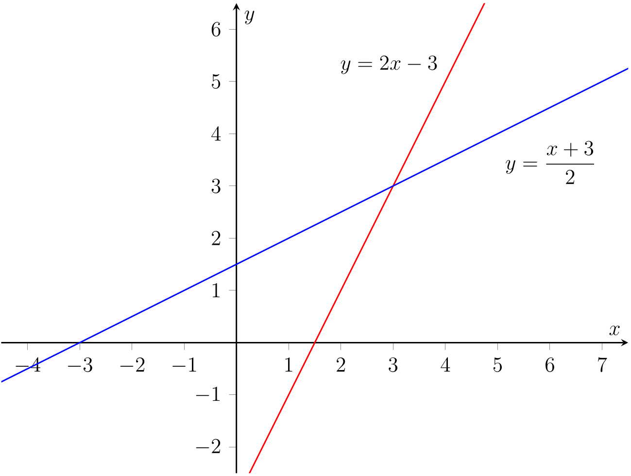
Fig. 4.15 Graph of \(y = 2x -3\) and \(y = \frac 12 x + \frac 32\)#
We see that the graphs of \(y = f(x)\) and \(y= f^{-1}(x)\) are reflections of one another in the line \(y = x\).
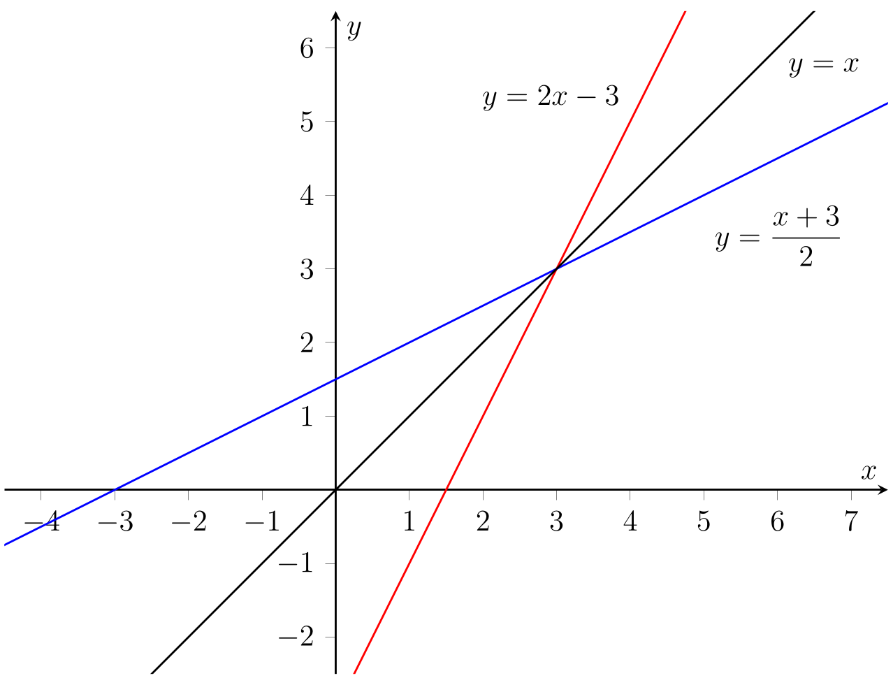
Fig. 4.16 Graph of \(y = 2x -3\), \(y = \frac 12 x + \frac 32\) and \(y=x\).#
In fact, this relation holds for all functions \(f\) and \(f^{-1}\). That is,
If \(f\) is a function with inverse \(f^{-1}\) then the graph of \(y=f^{-1}(x)\) is obtained from the graph of \(y=f(x)\) by reflecting it in the line \(y=x\).
To see why, imagine the graph of \(y=f(x)\) is drawn on a transparent sheet. If the sheet is turned over so that the \(x\)-axis and the \(y\)-axis are interchanged then the graph is reflected in the line \(y=x\). Now, since the relationship \(y=f(x)\) still holds we see that \(x=f^{-1}(y)\). If we then re-label the axes in the conventional way, with \(x\) horizontal and \(y\) vertical, we see that the graph now represents \(y=f^{-1}(x)\), as required.
Exercise
The function \(f\) is given by \(f(x) = 1 -3x\).
Find \(f^{-1}\).
Sketch the graphs of \(y = f(x)\) and \(y = f^{-1}(x)\) on the same diagram. Add the straight line \(y = x\) and check the reflection property.
Solution
We have \begin{align*} y = 1-3x & so & y +3x = 1\ & so & 3x = 1-y\ & so & x = \frac{1-y}{3}. \end{align*} Hence \(f^{-1}(x) = \frac{1-x}{3}\).
We sketch the graphs of \(f\) and \(f^{-1}\) on the same axis.
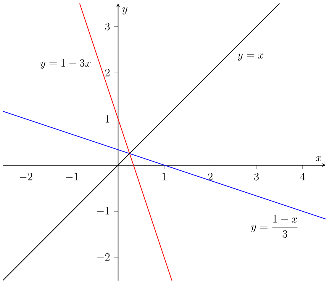
Fig. 4.17 Graph of the function \(f(x) = 1 -3x\) and its inverse \(f^{-1}(x) = \frac{1-x}{3}\).#
We see that the graphs of \(y=f(x)\) and \(y=f^{-1}(x)\) are indeed reflections in the line \(y=x\).
Exercise
Find the inverses of the following functions:
(i) \(f(x) =\displaystyle 12 - \frac 12 x\);
(ii) \(f(x) = \displaystyle \frac 12(x-3)\);
(iii) \(f(x) = \displaystyle \frac{2x+1}{5} \);
(iv) \(f(x) = \displaystyle \frac{7-3x}{10}\);
(v) \(f(x) = \displaystyle\frac 59(x-32)\);
(vi) \(f(x) =180(x-2)\);
(vii) \(f(x) = \displaystyle 2\pi x\);
(viii) \(f(x) = \displaystyle \frac{5(x+7)}{3} -9\);
(ix) \(f(x) = \displaystyle \frac 1{x-3}~~x \neq 3 \);
(x) \(f(x) = \displaystyle \frac 1{2x+1}~~x \neq \frac 12\);
(xi) \(f(x) = \displaystyle \frac 3{4-x}~~x\neq 4\);
(xii) \(f(x) = \displaystyle \frac{2x}{1+x}~~x \neq -1\).
4.5.2. Composing \(f\) and \(f^{-1}\)#
Recall the defining property of the inverse function from earlier, namely that \(y = f(x)\) if and only if \(x = f^{-1}(y)\). We return to Example 4.8 where the function \(f\) was given by \(f(x) = \frac{3x-1}{x+2}\). We found that \(f^{-1}(x) = \frac {1+2x}{3-x}\). We will investigate what happens if we compose \(f\) and \(f^{-1}\) in this case. Firstly, we have
Thus \(f^{-1}(f(x))=x\). Similarly, we get
Thus \(f(f^{-1}(x))=x\) as well. Again, this is no coincidence; that is, in general we have
for any function \(f\) with inverse \(f^{-1}\) we have \(f^{-1}(f(x)) = x\) and \(f(f^{-1}(x)) = x\).
4.5.3. Some functions do not have an inverse#
There are many functions that do not have an inverse. Let’s have a look why.
Example 4.10
Consider the function \(f(x) = x^2\). If we try to solve \(f(x) = 4\) for \(x\) we get \(x^2 = 4\) and we find two solutions, namely \(x=2\) and \(x=-2\). This can be seen on the graph below. The same goes for solving \(f(x) = 1\).
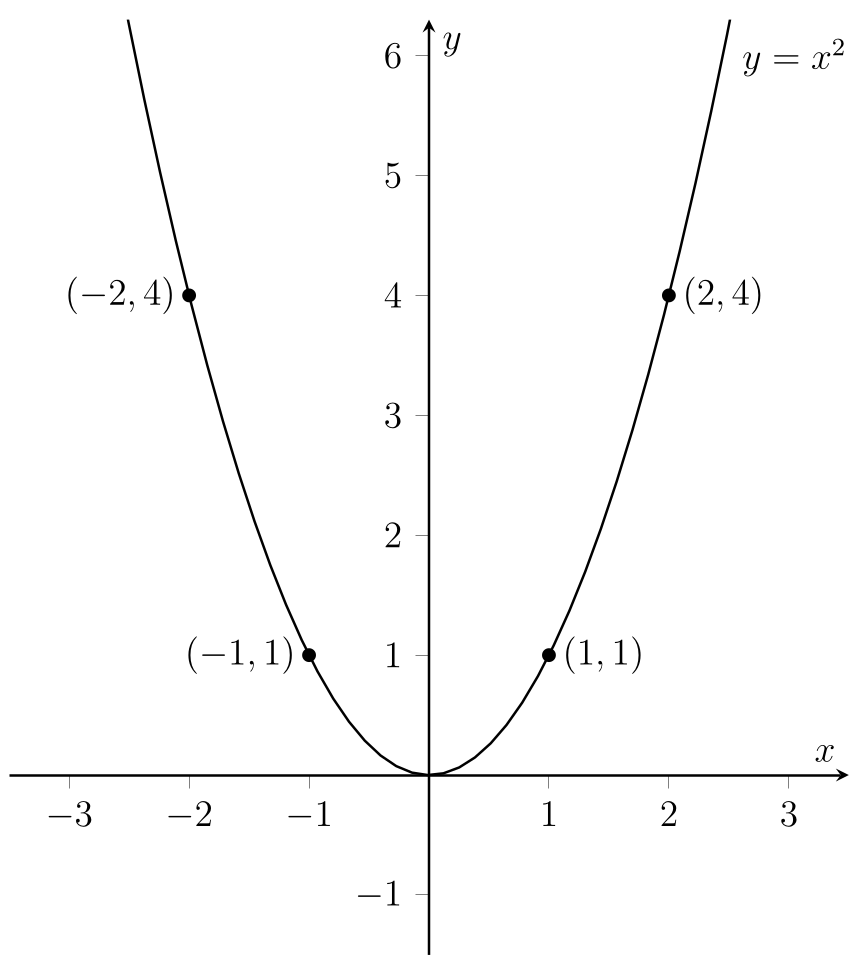
Fig. 4.18 Graph of \(y=x^2\), with points \((\pm 1,1)\) and \((\pm 2,4)\) marked.#
So we have no chance of finding an inverse function. Why? Well, if we did find a function \(f^{-1}\) then evaluating \(f^{-1}(4)\) would give \(\pm 2\) — that is, we’d get two values out. But one of the important properties of a function is that it only gives one output for each input.
So the function \(f(x) = x^2\) does not have a straightforward inverse. However, by thinking about our domain carefully we can create something like an inverse for \(f\).
We consider the related function \(g\) with \(g(x) = x^2\) (again) but domain \(\{ x\in\mathbb{R}:x \geq 0\}\). This has graph as shown below.
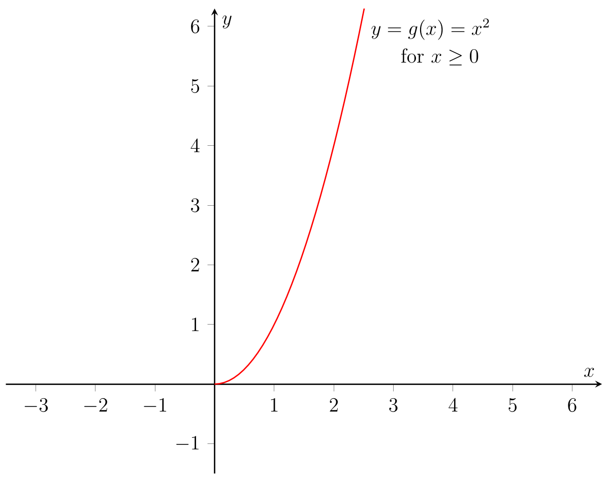
Fig. 4.19 Graph of \(y=x^2\), with domain restricted to \(x\geq 0\).#
Now we can see that, given non-negative number \(y\) we can find a unique value of \(x\) in the domain such that \(g(x)=y\). That is, we can now find an inverse function for \(g\). Note that if we reflect the graph of \(y=g(x)\) in the line \(y=x\) we get the graph for \(y=g^{-1}(x)\) as shown below.
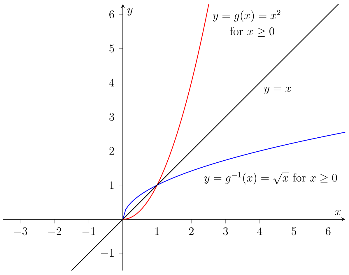
Fig. 4.20 Graph of \(y=x\), \(y=x^2\) for \(x\geq 0\), and \(y=\sqrt x\) for \(x\geq 0\).#
We call \(g\) the the positive square root function and write \(g^{-1}(x)=\sqrt{x}\) with domain \(\{x\in\mathbb{R}~:~x\geq 0\}\). We are, of course, already familiar with this!
Note that we have to be very careful about the domains in this case:
\(y = x^2\) and \(x \geq 0\) if and only if \(x = \sqrt{y}\).
4.6. Trigonometric Functions and Their Graphs#
Note that this part of the course is degree-free. We will always use radians here.
4.6.1. The functions \(y = \sin x\) and \(y = \cos\)#
Recall the (geometrical) definition of \(\sin \theta\) and \(\cos\theta\). On a pair of coordinate axes we draw a circle of radius \(1\) with its centre at the origin. We draw a radius of the circle at an angle \(\theta\), measured anti-clockwise from the \(x\)-axis. Let \(P\) be the point where this radius meets the circle. We define \(\sin \theta\) to be the \(y\)-coordinate and \(\cos \theta\) the \(x\)-coordinate of \(P\).
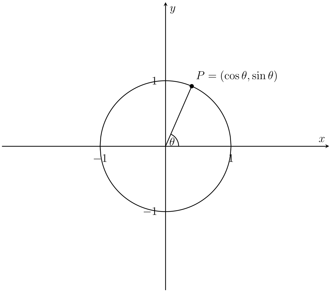
Fig. 4.21 Trigonometric circle, with \(P=(\cos\theta,\sin\theta)\) marked#
Note that we can think of \(\cos\) and \(\sin\) as functions with domain \(\mathbb{R}\) and codomain \(\mathbb{R}\). Shortly we will draw the graphs of \(\sin\) and \(\cos\) and see that they both have range
Note
From the definition, it is clear that every time we make a full revolution we get the same values for \(\sin\theta\) and \(\cos\theta\). That is, \(\sin (\theta+2\pi)=\sin(\theta)\) and \(\cos(\theta+2\pi)=\cos\theta\). In fact, we can add any multiple of \(2\pi\) on, both negative and positive and the result still holds.
For any integer \(k\) we have \(\sin(\theta+2k\pi)=\sin\theta\) and \(\cos(\theta+2k\pi)=\cos\theta\).
So \(\sin \theta\) and \(\cos \theta\) repeat every \(2\pi\) radians. We say that \(\sin\) and \(\cos\) are periodic with period \(2\pi\). We draw the graphs of \(y=\sin x\) and \(y=\cos x\) below.
.png)
Fig. 4.22 Graph of \(y=\sin x\)#
.png)
Fig. 4.23 Graph of \(y=\cos x\)#
As claimed earlier, we see from their graphs that the ranges of both \(\sin\) and \(\cos\) are \(\{ y\in\mathbb{R}:-1 \leq y \leq 1\}\) (since these are the values of \(y\) horizontally in line with the graph). We also see that \(\sin x = 0\) if and only if \(x = k\pi\) where \(k\) is any integer; similarly \(\cos x = 0\) if and only if \(x = \frac{\pi}{2}+k\pi\) where \(k\) is any integer.
The important facts to remember for \(y = f(x) = \sin x\) are:
The domain of \(\sin x\) is \(\mathbb{R}\)
The range of \(\sin x\) is \(\{ y \in \mathbb{R}:- 1 \leq y \leq 1\}\)
\(\sin x\) is periodic with period \(2\pi\)
\(\sin x = 0\) if and only if \(x = k\pi\) for some \(k \in \mathbb{Z}\)
\(\sin x = 1\) if and only if \(x = \frac \pi 2 + 2\pi k\) for some \(k \in \mathbb{Z}\)
\(\sin x = -1\) if and only if \(x = - \frac \pi2 + 2\pi k\) for some \(k \in \mathbb{Z}\)
For \(y = f(x) = \cos x\), the important facts to remember are:
The domain of \(\cos x\) is \(\mathbb{R}\)
The range of \(\cos x\) is \(\{y \in \mathbb{R}:- 1 \leq y \leq 1\}\)
\(\cos x\) is periodic with period \(2\pi\)
\(\cos x = 0\) if and only if \(x = \frac \pi 2 + k\pi\) for some \(k \in \mathbb{Z}\)
\(\cos x = 1\) if and only if \(x = 2\pi k\) for \(k \in \mathbb{Z}\)
\(\cos x = - 1\) if and only if \(x = \pi (2k infinite+1)\) for \(k \in \mathbb{Z}\)
Remark 4.1
One way to think about the functions \(y = \sin x\) and \(y = \cos x\) is to think of them in terms of their Taylor series. You will encounter this concept later in your course. The amazing fact is that one can work out \(y = \sin x\) and \(y = \cos x\) as an ** sum, or “infinite degree” polynomial. We have
while
where for any positive integer \(n\) we have \(n! = 1 \times 2 \times 3 \times \ldots\times n\) and \(0! = 1\). The symbol \(\sum\) means that one needs to add up each term while \(n\) runs through all the non-negative integers. In fact, your calculator uses finite approximations of these series to find values for the trigonometric functions. One can then define \(\pi\) via \(\frac \pi 2\) is the first positive zero of the function \(y = \cos x\).
4.6.2. The function \(\tan\)#
Recall that, having defined \(\sin\) and \(\cos\) already we define a function \(\tan\) by
You should have already seen in MAS002 that the graph of \(y=\tan x\) is as follows.
.png)
Fig. 4.24 Graph of \(y=\tan x\).#
We’ll have a look why this works by thinking about the graphs of \(y=\sin x\) and \(y=\cos x\).
The graph of \(y=\tan x\)#
Step 1: We have \(\tan x = 0\) if and only if \(\frac{\sin x}{\cos x} = 0\) which is the case if and only if \(\sin x=0\). That is, \(\tan x=0\) when \(x=k\pi\) for any integer \(k\).
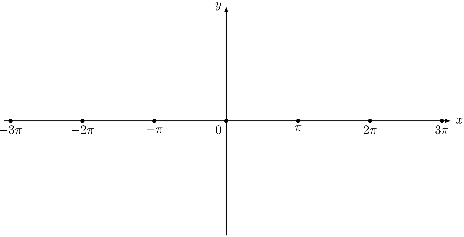
Fig. 4.25 Axes with the zeros of \(\tan x\) marked.#
Step 2: Note that where \(\cos x = 0\) we can’t divide by \(\cos x\) so that \(\tan x= \frac{\sin x}{\cos x}\) is undefined. Hence \(\tan x\) is undefined at \(x=\frac{\pi}{2}+k\pi\) for any integer \(k\). We mark these points on a set of axes. We then draw the vertical lines through these points as our graph is not allowed to touch or cross these lines.
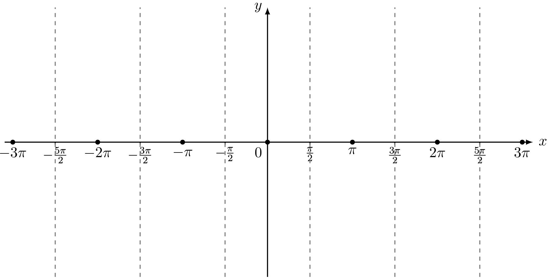
Fig. 4.26 Axes with the zeros and vertical asymptotes of \(y=\tan x\) marked#
Step 3: Let \(x\) start at \(0\) and increase to \(\frac \pi 2\). As \(x\) increases (gets bigger), \(\sin x\) increases from \(0\) to \(1\) and \(\cos x\) decreases from \(1\) down to \(0\). Hence \(\tan x=\frac{\sin x}{\cos x}\) increases. As \(x\) approaches \(\frac \pi 2\) \(\sin x\) approaches \(1\) and \(\cos x\) approaches \(0\). This means that \(\tan x\) will get bigger and bigger with no bound; that is, \(\tan x\) approaches \(+\infty\) (plus infinity).
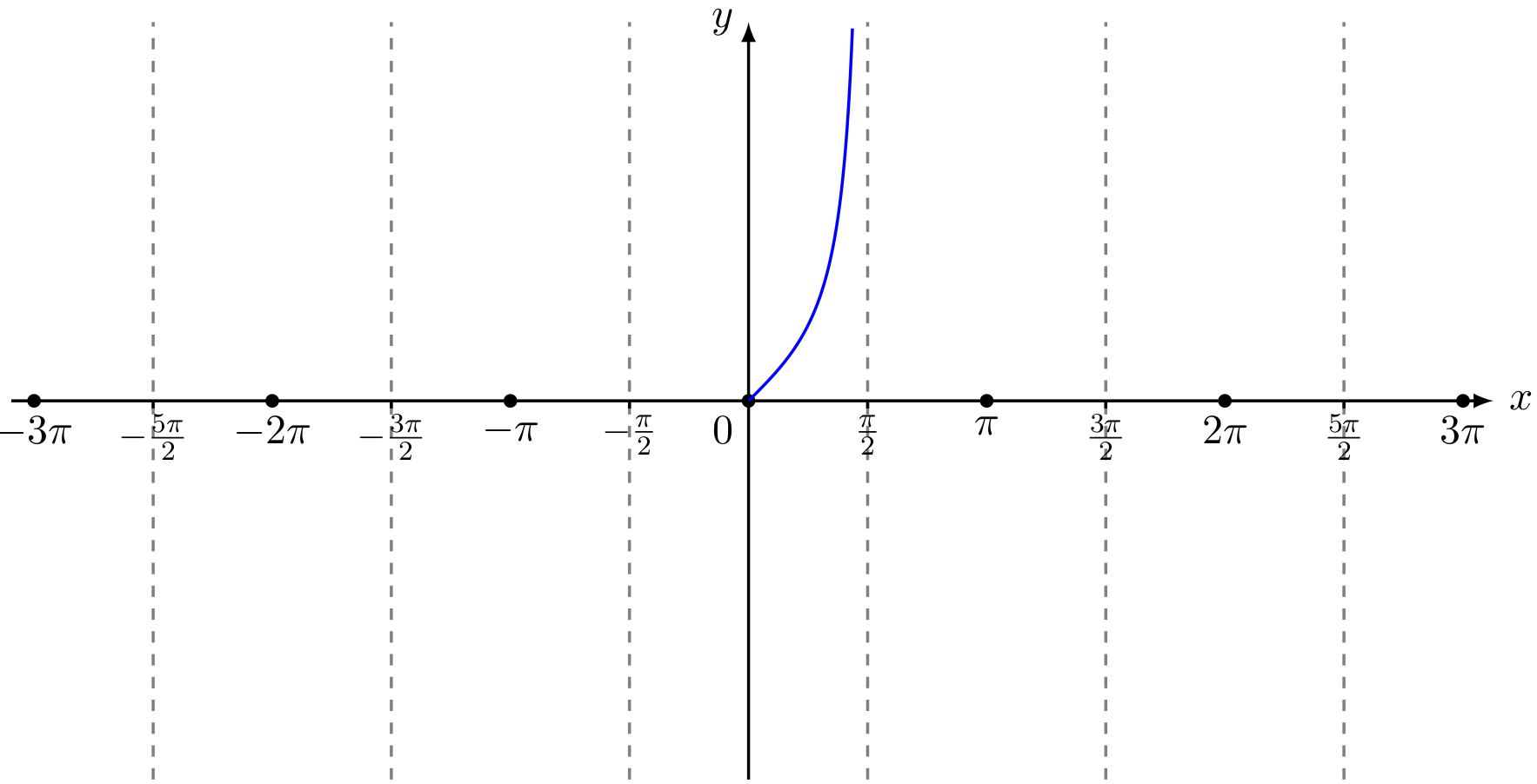
Fig. 4.27 Axes with the zeros and vertical asymptotes, as well as \(y=\tan x\) for \(0\leq x<\frac{\pi}{2}\).#
Step 4: Now let \(x\) start at \(0\) and decrease to \(- \frac \pi 2\). As \(x\) decreases, \(\sin x\) decreases from \(0\) to \(-1\) and \(\cos x\) decreases from \(1\) down to \(0\). Hence \(\tan x\) becomes negative and decreases. As \(x\) approaches \(\frac \pi 2\) \(\sin x\) approaches \(-1\) and \(\cos x\) approaches \(0\). Hence \(\tan x\) approaches \(-\infty\) (minus infinity).
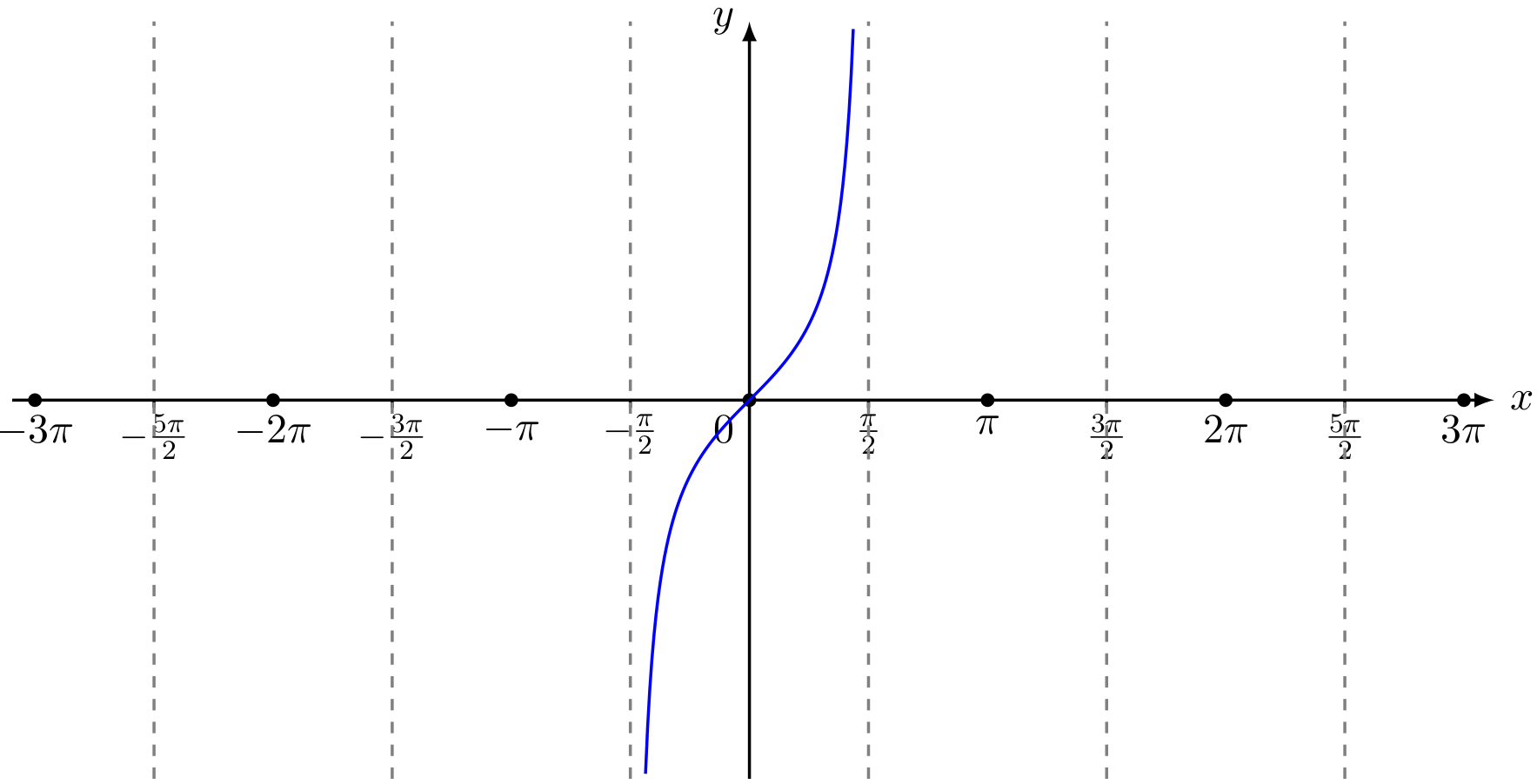
Fig. 4.28 Axes with the zeros and vertical asymptotes, as well as \(y=\tan x\) for \(-\frac{\pi}{2}<x<\frac{\pi}{2}\).#
Step 5: We can repeat similar arguments for \(\frac{\pi}{2}< x< \pi\) and \(-\pi< x< -\frac{\pi}{2}\). Also, since \(\sin x\) and \(\cos x\) repeat every \(2\pi\) radians, so will \(\tan x\) and we get the familiar graph below.
Fig. 4.29 Graph of \(y=\tan x\)#
The important facts to remember about \(y = f(x) = \tan x\) are
The domain of \(\tan x\) is \(\{ x \in \mathbb{R}:x \neq \frac{\pi}{2}+k\pi \mbox{ for } k \in \mathbb{Z}\}\)
The range of \(\tan x\) is \(\mathbb{R}\)
\(\tan x\) is periodic with period \(\pi\)
\(\tan x = 0\) if and only if \(x = \pi k\) for some \(k \in \mathbb{Z}\).
4.6.3. Reciprocal trigonometric functions#
As well as the standard three trig functions \(\sin(x)\), \(\cos(x)\) and \(\tan(x)\), you will to know the graphs of the so-called \emph{reciprocal trig functions}, \(\text{cosec}(x)\), \(\sec(x)\) and \(\cot(x)\).
In maths, the word reciprocal means “1 over”, and the reciprocal trig functions are none other than “1 over” the standard three trig functions.
Definition 4.2 (Reciprocal trig functions)
We define
There is a monica for remembering which way round they go. Look at the third letter of each of \( \text{cosec}\), \(\sec\) and \(\cot\). This will give you the first letter of the function it is the reciprocal of.
The graph of \(y= \text{cosec}(x)\)#
Since \( \text{cosec}(x)=\frac{1}{\sin(x)}\), its graph will have vertical asymptotes whenever \(\sin(x)=0\). So \(y= \text{cosec}(x)\) will go to \(\pm\infty\) when \(x=0,\pm \pi,\pm 2\pi,\ldots\).
We also know that if \(\sin(x)=\pm 1\), then \( \text{cosec}(x)=\frac{1}{\pm 1}=\pm 1\). That is,
\(y= \text{cosec}(x)=1\) when \(x=\frac{\pi}{2}+2k\pi\), \(k\in\mathbb{Z}\).
\(y= \text{cosec}(x)=-1\) when \(x=-\frac{\pi}{2}+2k\pi\), \(k\in\mathbb{Z}\).
It must also be positive where \(\sin(x)\) is positive, and negative where \(\sin(x)\) is negative.
This is enough information to be able to sketch the graph of \(y= \text{cosec}(x)\):
.png)
Fig. 4.30 raph of \(y= \text{cosec} x=\frac{1}{\sin(x)}\).#
The graph of \(y=\sec(x)\)}.#
Just as \(y=\cos(x)\) is a shifted version of \(y=\sin(x)\) the graph of \(y=\sec(x)=\frac{1}{\cos(x)}\) can be obtained by translating the graph of \(y= \text{cosec}(x)=\frac{1}{\sin(x)}\) by \(\frac{\pi}{2}\) in the negative \(x\) direction:
.png)
Fig. 4.31 Graph of \(y=\sec x=\frac{1}{\cos(x)}\).#
Comparing with the graph of \(y=\cos(x)\) (c.f. Fig. 4.23), we note that
\(\sec(x)=1\) whenever \(\cos(x)=1\), i.e.~at even multiples of \(\pi\),
\(\sec(x)=-1\) whenever \(\cos(x)=-1\), i.e.~at odd multiples of \(\pi\),
\(\sec(x)\) is positive whenever \(\cos(x)\) is positive (and negative whenever it is negative)
\(\sec(x)\) has a vertical asymptote (i.e.~tends to \(\pm\infty\)) whenever \(\cos(x)=0\)
\(\sec(x)\) itself is never zero.
The graph of \(y=\cot(x)\).#
Note that since \(y=\cot(x)=\frac{1}{\tan(x)}\), and since \(\tan(x)=\frac{\sin(x)}{\cos(x)}\), we have
We could use this equation to decide where \(y=\cot(x)\) should have vertical asymptotes and where it should cross the axis, but in fact we can do one better. It turns out that the graph of \(y=\cot(x)\) can be understood as a transformed version of \(y=\tan(x)\).
Spefically, we claim that
for all \(x\in\mathbb{R}\).
To see why this is indeed the case, observe that
Indeed, the graph of \(y=\cos(x)\) can be transformed into \(y=\sin(x)\) by translating by \(\frac{\pi}{2}\) in the positive \(x\) direction. Similarly,
— if we shift \(y=\sin(x)\) by \(\frac{\pi}{2}\) in the positive \(x\) direction, and then reflect in the \(x\)-axis, we recover the graph of \(y=\cos(x)\).
Substituting these two equations into (4.1), we get
as desired.
Equation (4.2) means we can obtain the graph of \(y=\cot(x)\) by shifting the graph of \(y=\tan(x)\) by \(\frac{\pi}{2}\) in the positive \(x\) direction, and then reflecting it in the \(x\)-axis. We get the following:
.png)
Fig. 4.32 Graph of \(y=\cot x=\frac{1}{\tan(x)}\).#
4.6.4. Inverse trigonometric functions#
The inverse of \(\sin\)#
If we look at the graph of \(y=\sin x\) we see that we will have a problem constructing an inverse function.
Fig. 4.33 Graph of \(y=\sin x\)#
As with \(y=x^2\) the problem is that more that one value of \(x\) give the same value of \(y\). We have to get around this problem by restricting the domain so that for each value of \(y\) in the range there is a precisely one value of \(x\) for which \(y=\sin x\). Obviously we want as big a domain as possible and it would be nice to include \(0\) as this is one of the easiest numbers. Thus we choose as domain \(\{x\in\mathbb{R}~:~-\frac{\pi}{2}\leq x\leq \frac{\pi}{2}\}\); that is we take consider just the values of \(x\) such that \(- \frac \pi2 \leq x \leq \frac \pi 2\). sinx for -pi/2≤x≤pi/2
restricted.png)
Fig. 4.34 Graph of \(y=\sin x\) for \(-\frac{\pi}{2}\leq x\leq \frac{\pi}{2}\)#
If we now reflect this graph in the line \(y = x\) we get the inverse function, which we denote by \(\sin^{-1}\) (or sometimes \(\arcsin\)).
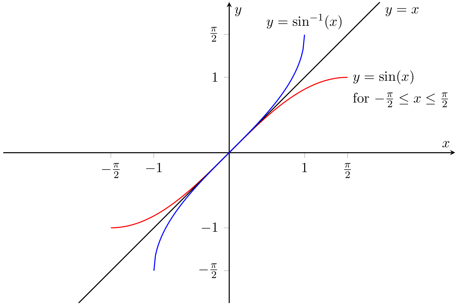
Fig. 4.35 Graph of the sine function and its inverse#
So the graph of \(y = \sin^{-1}(x)\) looks like
.png)
Fig. 4.36 Graph of \(y=\sin^{-1}x\)#
We see that \(\sin^{-1} x\) has domain \(\{ x\in\mathbb{R}:-1 \leq x \leq 1\}\) and range \(\{ y\in\mathbb{R}:-\frac \pi2 \leq y \leq \frac \pi 2\}\). That means we have the following relationship.
If \(-\frac \pi 2 \leq x \leq \frac \pi 2\) then \(y = \sin x\) if and only if \(x = \sin^{-1}y\).
You may like to check that, using the \(\sin^{-1}\) or \(\arcsin\) button on your calculator only works if you put in value between \(-1\) and \(1\) and gives out values in the range \(-\frac{\pi}{2}\) to \(\frac{\pi}{2}\).
The inverse of \(\cos\)#
We have to do a similar thing as we did to find \(\sin^{-1}\). We want to restrict the domain so as to find a part of \(\cos x\) such that any horizontal line meets it at at most one point. We choose the domain \(\{x\in\mathbb{R}~:~0\leq x\leq \pi\}\).
restricted.png)
Fig. 4.37 \(y=\cos x\) for \(0\leq x\leq \pi\)#
If we reflect this in the line \(y = x\) we get the graph of \(y=\cos^{-1}(x)\) (sometimes written \(y=\arccos x\)).
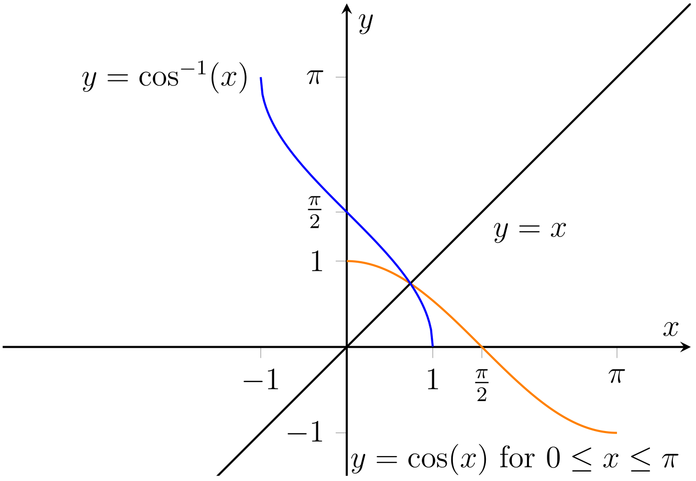
Fig. 4.38 Graph of the cosine function and its inverse#
So the graph of the inverse function of \(y = \cos x\) looks like y = cos^{-1}(x)
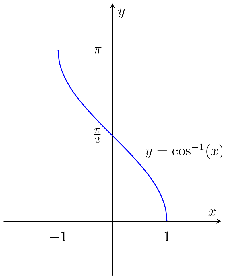
Fig. 4.39 Graph of the inverse cosine function#
We see that \(\cos^{-1} x\) has domain \(\{ x\in\mathbb{R}:-1 \leq x \leq 1\}\) and range \(\{ y\in\mathbb{R}:0 \leq y \leq \pi \}\). We have the relationship below.
If \(0\leq x\leq \pi\) then \(y = \cos x\) if anf only if \(x = \cos^{-1}y\).
Again, check that your calculator uses the function in this way.
The Inverse of \(\tan\)#
We do a similar thing as for \(\sin\) and \(\cos\). We want to restrict the domain of \(\tan x\) so that any horizontal line meets the graph of \(y=\tan x\) in at most one point. We restrict the domain to \(\{x\in\mathbb{R}~:~-\frac \pi 2 <x<\frac \pi 2\}\).
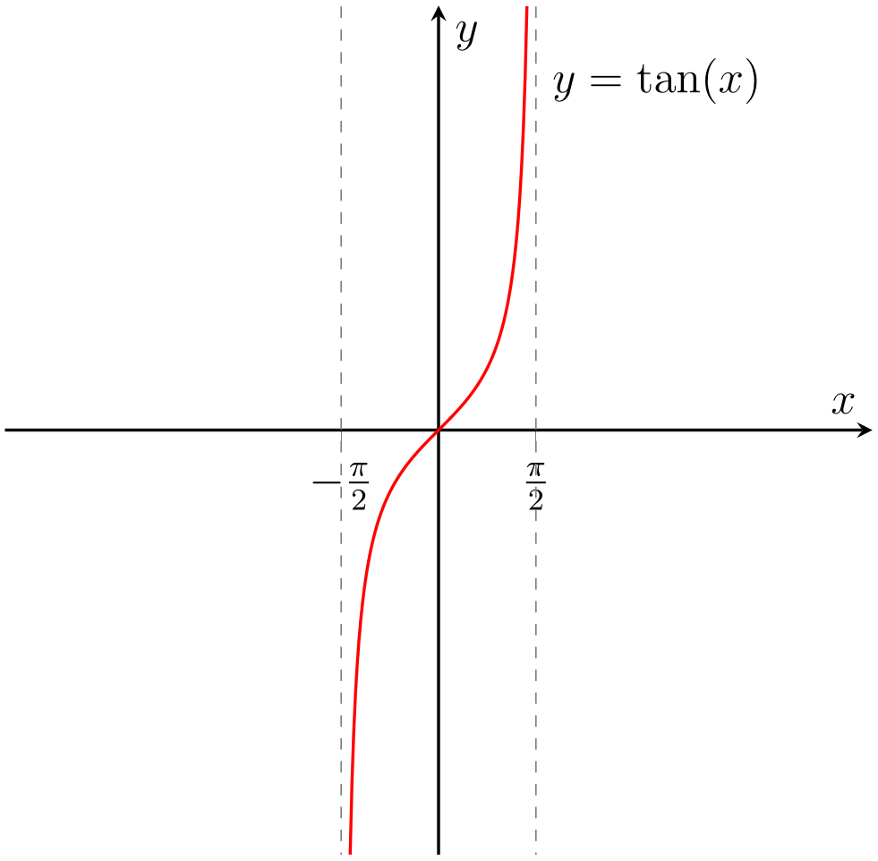
Fig. 4.40 \(y=\tan x\) for \(-\frac{\pi}{2}<x<\frac{\pi}{2}\)#
Reflecting this in the line \(y = x\) we get the graph of \(y=\tan^{-1}(x)\) (sometimes written as \(\arctan(x)\)).
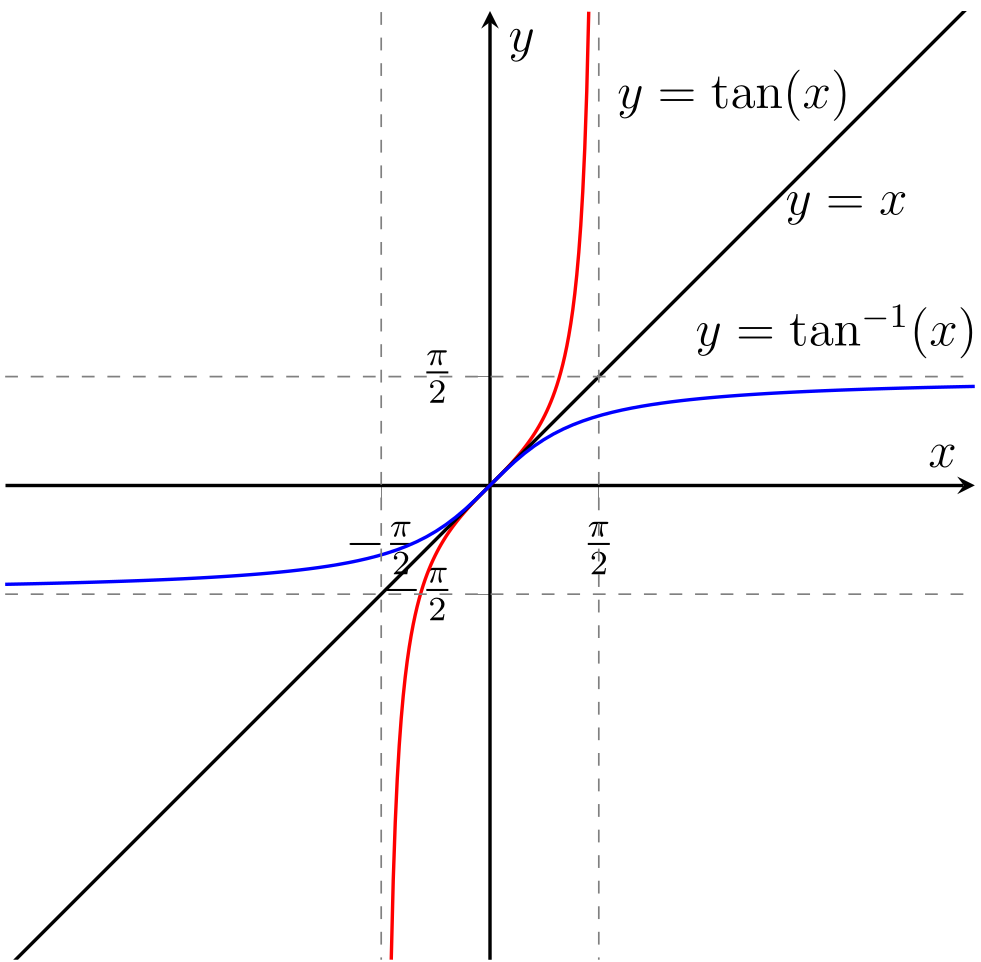
Fig. 4.41 Graph of the tan function and its inverse#
We see that \(\tan^{-1} x\) has domain \(\mathbb{R}\) and range \(\{ y\in\mathbb{R}:-\frac \pi2 < y < \frac\pi2 \}\). We have the relationship below.
If \(-\frac \pi 2 < x < \frac\pi2\) then \(y = \tan x\) if and only if \(x = \tan^{-1}y\).
Again, you might like to check that your calculator agrees with this.
Note that when \(x \rightarrow \infty\) then \(\tan^{-1} x \rightarrow \frac \pi 2\); and when \(x \rightarrow - \infty\) then \(\tan^{-1} x \rightarrow - \frac \pi 2\).
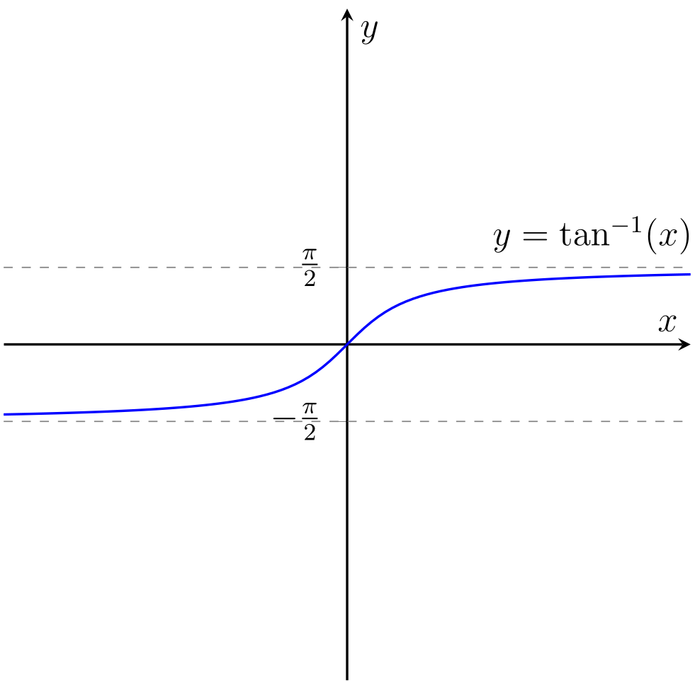
Fig. 4.42 Graph of \(y=\tan^{-1}x\)#
Warning
Note that \(\sin^{-1} x\) is not the same as \(\frac 1{\sin x}\), \(\cos^{-1} x\) is not the same as \(\frac 1{\cos x}\) and \(\tan^{-1} x\) is not the same as \(\frac 1{\tan x}\)! These are common mistakes.
4.7. Transforming the Graphs of Trigonometric Functions#
In Section 2.5.3 we saw how to transform the graphs of quadratics, moving them up and down, left and right and even stretching them. We can use the same methods to do this for the trigonometric functions.
Recall the graph of \(y = \sin x\).
Fig. 4.43 Graph of \(y=\sin x\).#
Note
It’s crucial to mark the values of the points where the graph crosses the \(x\)-axis, and the value of the amplitude on the \(y\)-axis. Otherwise we may not see much a difference in the graphs we obtain!
We have the following results using the same reasoning as earlier in the course.
Remark 4.2
Let \(a\) be any non-zero real number.
To sketch the graph of \(y = \sin x + a\) we take the graph of \(y = \sin x\) and move it up by a distance of \(a\) in the positive \(y\)-direction.
To sketch the graph of \(y = a \sin x\) (for \(a>0\)), we stretch the graph of \(y = \sin x\) by a factor of \(a\) in the \(y\)-direction. Note that the “wave” now has amplitude \(a\).
To sketch the graph of \(y = - \sin x\) we reflect the graph of \(y = \sin x\) in the \(x\)-axis.
To sketch the graph of \(y = \sin \left(x-a\right)\) we move the graph of \(y = \sin x\) by a distance of \(a\) in the positive \(x\)-direction. Note that in sketching such graphs your will be expected to denote the interesting points of the graph, such as crossings of the axes and amplitudes.
Example 4.11
Sketch the graph of \(y = \sin (5x)\).
Solution.
Let’s think about where \(\sin(5x)=0\). Note that \(\sin (x)=0\) when \(x=k\pi\) for any integer \(k\in\mathbb{Z}\) so \(\sin(5x)=0\) when \(5x=k\pi\), that is \(x=\frac{k\pi}{5}\). So the zeros of \(y=\sin (5x)\) are much closer together. In fact, what has happened is that we have squashed the graph of \(y=\sin x\) closer together, by a factor of \(5\). Perhaps a more helpful way to think about it is that we have stretched the graph of \(y=\sin x\) in the \(x\)-direction by a factor of \(\frac 15\). The oscillations have become more rapid — \(\sin x\) has period \(2\pi\) whereas \(\sin (5x)\) has period \(\frac{2\pi}5\).
We also know that \(\sin x = 1\) if and only if \(x = \frac \pi 2 + 2\pi k\) for \( k \in \mathbb{Z}\). Thus \(\sin (5x) = 1\) if and only if \(5x = \frac \pi 2 + 2\pi k\) for \( k \in \mathbb{Z}\). And this means that \(\sin (5x) = 1\) if and only if \(x = \frac \pi {10} + \frac{2\pi}5 k\) for \( k \in \mathbb{Z}\).
Further \(\sin x = - 1\) if and only if \(x = -\frac \pi 2 + 2\pi k\) for \( k \in \mathbb{Z}\). Thus \(\sin (5x) = 1\) if and only if \(5x = -\frac \pi 2 + 2\pi k\) for \( k \in \mathbb{Z}\). And this means that \(\sin (5x) = 1\) if and only if \(x = - \frac \pi {10} + \frac{2\pi}5 k\) for \( k \in \mathbb{Z}\).
.png)
Fig. 4.44 Graph of \(y=\sin(5x)\)#
Note
You are expected to mark these points in your graph, but obviously, if I try this here on the graphic, it will be far too messy. So if you have too many points to sensibly put into your graph, state them before or after your graph and indicate them on your graph.
Example 4.12
Sketch the graph of \(y = \sin (-x)\).
Solution.
Given any \(x\)-value, the value of \(\sin(-x)\) is just the value of \(\sin x\) evaluate at \(-x\). It follows that, the graph of \(y=\sin (-x)\) will just be the graph of \(y=\sin x\) reflected in the \(y\)-axis. That is, we have the following.
.png)
Fig. 4.45 Graph of \(y=-\sin(x)\)#
Piecing these results together, we see that they work for any function, not just \(\sin\). In other words.
Summary: Transforming the graph of \(y=f(x)\)
Given a function \(f:\mathbb{R}\to \mathbb{R}\) and a non-zero real number \(a\), then
the graph of \(y=f(x)+a\) is the graph of \(y=f(x)\) shifted in the positive \(y\)-direction by a distance of \(a\);
the graph of \(y=f(x-a)\) is the graph of \(y=f(x)\) shifted in the positive \(x\)-direction by a istance of \(a\);
if \(a>0\) the graph of \(y=af(x)\) is the graph of \(y=f(x)\) stretched in the positive \(y\)-direction by a factor of \(a\);
if \(a>0\) the graph of \(y=f(ax)\) is the graph of \(y=f(x)\) stretched in the positive \(x\)-direction by a factor of \(\frac{1}{a}\);
the graph of \(y=-f(x)\) is the graph of \(y=f(x)\) reflected in the \(x\)-axis;
the graph of \(y=f(-x)\) is the graph of \(y=f(x)\) reflected in the \(y\)-axis.
You need to be able to make such transformations of graphs, so learn the rules or understand how to derive them.
Exercise
Sketch the graphs of
(i) \(y = \displaystyle \cos (2x)\);
(ii) \(y =\sin (\frac 12 x)\);
(iii) \(y =\sin (\frac 32x)\);
(iv) \(y = \cos(x+\frac \pi 3)\);
(v) \(y = \sin (x - \frac \pi2)\);
(vi) \( y = \displaystyle 3\cos x; y = 2\cos (\frac 12x)\);
(vii) \(y = -\frac 12 \sin(2x)\);
(viii) \(y = 1-2\sin x\);
(ix) \( y = \displaystyle 3+2\cos (3x) \);
(x) \(y = \displaystyle \frac{1}{2+\sin x}\);
(xi) \(y = \displaystyle \frac 1{4-3\cos x}\).
Exercise
Sketch the graph of \(y = 4\cos (x - \frac \pi6)\).
Solution.
We start with the graph of \(y = \cos x\).
Fig. 4.46 Graph of \(y=\cos(x)\)#
Using our rules, we first translate \(y = \cos x\) by \(\frac \pi6\) in the positive \(x\)-direction to get the graph of \(y=\cos\left(x -\frac{\pi}{6}\right)\).
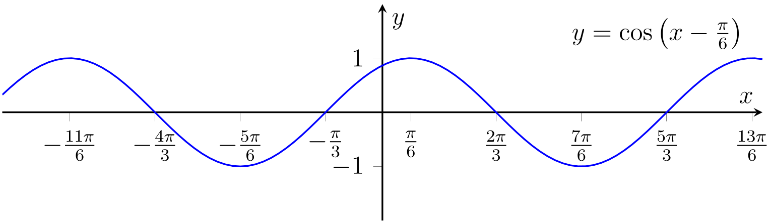
Fig. 4.47 Graph of \(y=\cos\left(x -\frac{\pi}{6}\right)\)#
Now we stretch the graph of \(y=\cos(x - \frac \pi6)\) in the \(y\)-direction by a factor of \(4\) to get the graph of \(y = 4\cos(x - \frac \pi6)\).
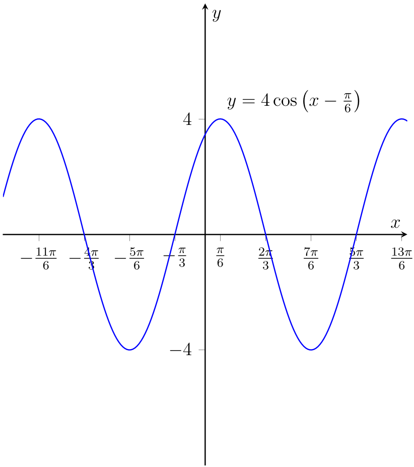
Fig. 4.48 Graph of \(y=4\cos\left(x-\frac{\pi}{6}\right)\).#
Note that the graph crosses the \(x\)-axis when \(\cos(x-\frac{\pi}{6})=0\), that is when \(x-\frac{\pi}{6}=\frac{\pi}{2}+k\pi\) (\(k\in\mathbb{Z}\)). Hence the zeros occur when \(x=\frac{\pi}{6}+\frac{\pi}{2} + k\pi=\frac{2\pi}{3} + k\pi\). We should also label the peaks and troughs. The peaks occur when \(\cos(x-\frac{\pi}{6})=1\); that is \(x-\frac{\pi}{6}=2k\pi\) so that \(x=\frac{\pi}{6}+2k\pi\) (\(k\in\mathbb{Z}\)). Similarly the troughs are when \(x-\frac{\pi}{6}=\pi+2k\pi\), that is when \(x=\frac{5\pi}{6}+2k\pi\) (\(k\in\mathbb{Z}\)). The place where the graph crosses the \(y\)-axis is more tricky, but you should be able to find it using the inverse \(\cos\) function (exercise!).
4.8. The Modulus Function#
Definition 4.3 (Modulus function)
We define the modulus function, denoted \(|x|\), by
We can define this more formally by
The number \(|x|\) is called the modulus of \(x\) or the absolute value of \(x\).
Example 4.13
We have \(|-2.7| = 2.7\) and \(|3.5| = 3.5\). We also see this on the real line below.
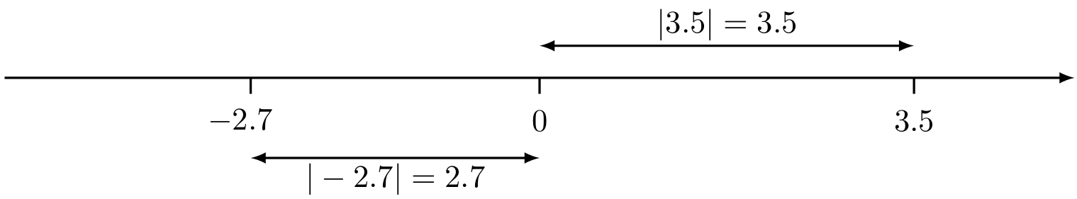
Fig. 4.49 The modulus of \(-2.7\) and \(3.5\) on the real line#
Note that we can informally think of the modulus function as “forgetting the minus sign”.
Exercise
Draw the graph of \(f(x) = |x|\).
Solution.
The graph of \(y=|x|\) is as follows.
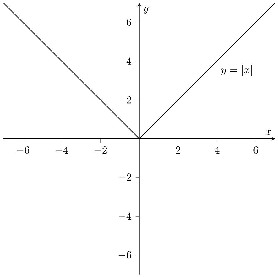
Fig. 4.50 Graph of \(y=|x|\)#