Differentiation

6. Differentiation#

6.1. Tangents and Gradients#

Recall that by the gradient of a curve at a point we mean the slope of the curve at that point. We can get an estimate of this in a number of ways. We illustrate how with an example.

Example 6.1

Consider the graph of $y = x^2$ shown below. Find the gradient of this curve at the point $(3,9)$.

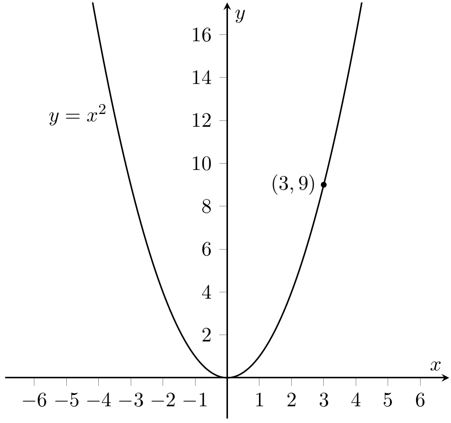
_images/graphx2.png — Fig. 6.1 Graph of $y=x^2$, with the point $(3,9)$ marked.#

6.1.1. Approximation Method I#

Draw the straight line through the point $(3,9)$ which is parallel to and just touches the curve at this point. This line is called the {\em tangent to the curve} at $(3,9)$. We find the gradient of the curve at $(3,9)$ by finding the gradient of this tangent line.

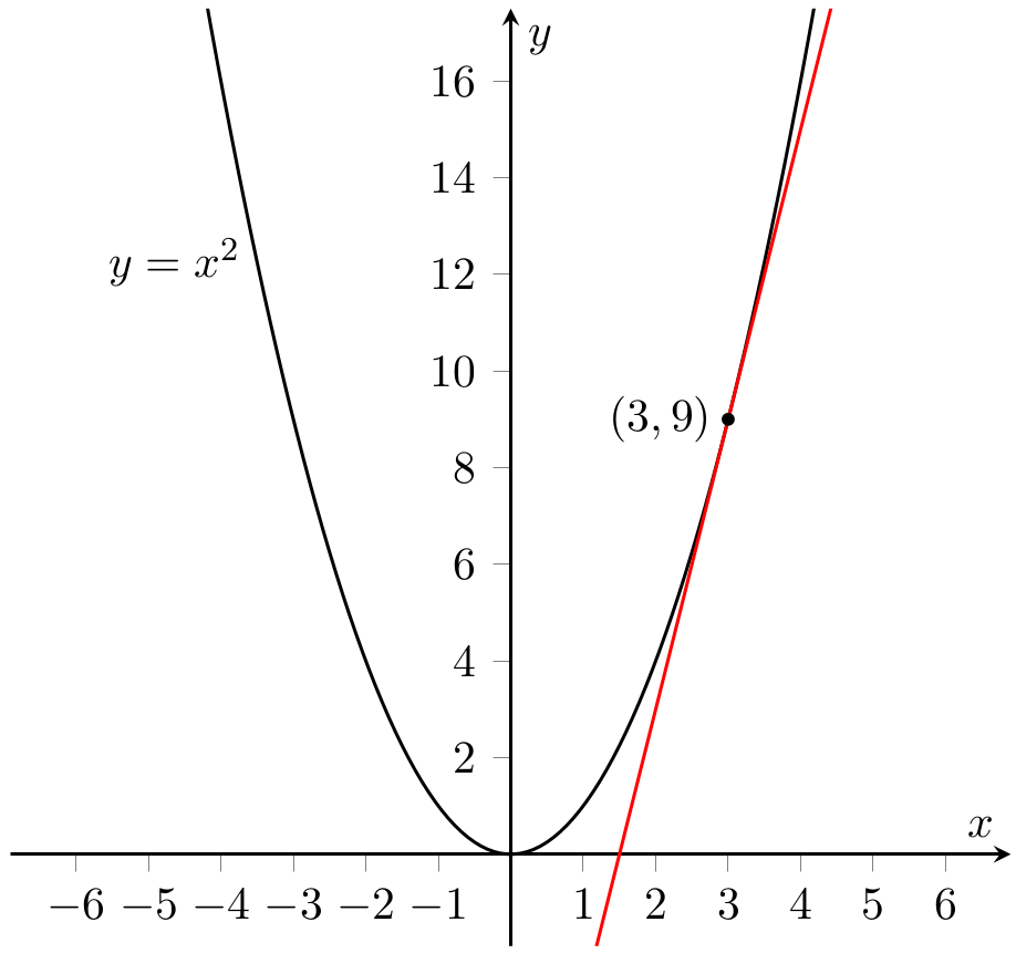
_images/graphx2tangent.png — Fig. 6.2 Graph of $y=x^2$ with tangent at $(3,9)$#

To find the gradient, $m$, of the tangent line we use the formula

\[ m = \frac{y_1-y_0}{x_1-x_0} \]

where $(x_1,y_1)$ and $(x_0,y_0)$ are any two points on the line. In our case, the tangent line will cut the $x$-axis at approximately $(1.5,0)$ so we can we take $(x_1,y_1)=(3,9)$ and $(x_0,y_0)=(1.5,0)$. Using the formula above we get

\[ m=\frac{9-0}{3-1.5}=\frac{9}{1.5}=6. \]

Hence the gradient of $y = x^2$ at $(3,9)$ is approximately $6$. Note that this method relies on drawing an accurate diagram to find some other points on the line, so is not a very good solution.

6.2. Approximation Method II#

We pick a second point, $(4,16)$ say, on the graph $y = x^2$ and consider the gradient of the straight line between this point and our original point $(3,9)$. Using the formula for the gradient, $m$, of this line with $(x_1,y_1)=(4,16)$ and $(x_0,y_0)=(3,9)$ we get

\[ m=\frac{16-9}{4-3} = 7. \]

This gives us another approximation of the gradient of our curve at $(3,9)$.

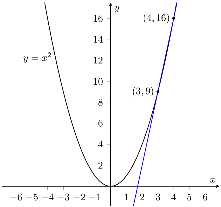
_images/graphx2tangentapprox.png — Fig. 6.3 Graph of $y=x^2$, with a line through $(3,9)$ and $(4,16)$.#

Now let the second point come nearer to $(3,9)$, for example $(3.1,9.61)$. The gradient, $m$, of the straight line between these two points is then

\[ m=\frac{9.61 - 9}{3.1-3} = \frac{0.61}{0.1} = 6.1. \]

_images/graphx2tangentapprox1.png — Fig. 6.4 Graph of $y=x^2$, with a line through $(3,9)$ and $(3.1,9.61)$.#

Moving our second point even closer, if we consider the point $(3.01,9.0601)$ we get:

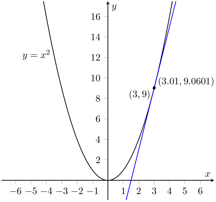
_images/graphx2tangentapprox2.png — Fig. 6.5 Graph of $y=x^2$, with a line through $(3,9)$ and $(3.01,9.0601)$ marked.#

The gradient, $m$, of the straight line between $(3,9)$ and $(3.01,9.0601)$ is

\[ m=\frac{9.0601 - 9}{3.01-3} = \frac{0.0601}{0.01} = 6.01. \]

We can then guess that the gradient of $y = x^2$ at $(3,9)$ is approximately $6$.

6.2.1. Precise Method — First Principles Differentiation#

We approach the problem using the ideas of the second method but turn the notion of choosing closer and closer points into proper maths.

We consider the point on the curve with $x$-coordinate $3+h$ where $h$ stands for a small positive number. Note that the $y$-coordinate is $(3+h)^2=9+6h+h^2$. We saw above that the gradient of $y = x^2$ at $(3,9)$ is approximately the gradient of the line joining this point with $(3,9)$, namely

\[ m=\frac{y_1-y_0}{x_1-x_0}=\frac{(9+6h+h^2) - 9}{(3+h) - 3} = \frac{6h+h^2}{h} = 6+h. \]

We also know that the approximation is better the smaller $h$ is.

If we let $h$ tend to zero (denoted $h \rightarrow 0$) we see that $m=6+h$ tends to $6$. It follows that the gradient of $y = x^2$ at $(3,9)$ is $6$.

We may also say that the rate of change of $y$ with respect to $x$ at $x=3$ is $6$.

Remark 6.1

The rate of change occurs in many practical applications, for example as rates of change in temperature. Some rates of change you may already be familiar with. For example, the rate of change of distance with respect to time is called velocity and the rate of change of velocity with respect to time is called acceleration. Needless to say, rates of change are a very important concept in mathematics, physics and engineering.

The third method above is often called differentiation by first principles.

Example 6.2

Find the gradient of $y = x^2$ at a typical point $(x,x^2)$ using first principles.

Solution.
As in the third method above, we start with the point $(x,x^2)$ and, for some small number $h$, the point $(x+h, (x+h)^2) = (x+h, x^2 + 2hx + h^2)$. The gradient of the straight line between these two points is

\[ m=\frac{(x^2+ 2hx + h^2) - x^2}{(x+h) - x} = \frac{2hx +h^2}{h} = 2x + h. \]

As $h \rightarrow 0$, we find that the gradient of the straight line is $2x+h$ which tends to $2x$.

Hence the gradient of $y = x^2$ at the typical point $(x, x^2)$ is $2x$.

Note

In our first example, we found that the gradient of $y=x^2$ at $(3,9)$ is $6$. This agrees with the above result on putting $x=3$ into the formula.

6.3. Differentiation#

Having used the standard quadratic to gain an intuition for differentiation from first principles, we are now ready to define it for a general function.

Definition 6.1

Given a function $f(x)$, the process of calculating

\[ \frac{f(x+h)-f(x)}{h} \]

as $h\rightarrow 0$ is known as {\em differentiation}, and we talk about ‘differentiating the function $f(x)$ with respect to $x$’.

Example 6.2 was an example of differentiation: all we are doing is finding the gradient of the curve $y=f(x)$ at the point $(x,f(x))$.

Example 6.3

Let $f(x)=3x+2$. Then $f(x+h)= 3(x+h)+2$, and so

\[ \frac{f(x+h)-f(x)}{h} = \frac{3(x+h)+2 - (3x+2)}{h}=\frac{3x+3h+2 - 3x-2}{h} = \frac{3h}{h} = 3. \]

So in this case, the quantity $\frac{f(x+h)-f(x)}{h}$ doesn’t even depend on $h$! Letting $h$ tend to zero gives

\[ \lim_{h\rightarrow 0}\frac{f(x+h)-f(x)}{h} = \lim_{h\rightarrow 0}3 = 3. \]

So differentiating $f(x)=3x+2$ gives $3$.

More generally, differentiating $f(x)$ (assuming it is possible) will always return a function of $x$ — the $h$ disappears in the limit as $h\rightarrow 0$. The function obtained by differentiating $f(x)$ is called the derivative of $f$ with respect to $x$, and denoted by $f'(x)$.

Note

Depending on how “nice” the function $f$ is, the differentiation process may not produce a proper function of $x$. However, for nearly every function we meet in this module, the derivative exists and is another function we are already familiar with.

Example 6.4

Let $f(x)=7x^2 + 5x$. Find the gradient of $y = f(x)$ at a typical point $(x,f(x))$.

Solution.
We use differentiation. If we put $x+h$ into our function $f$ we get that

\[\begin{align*} f(x+h) &= 7(x+h)^2 + 5(x+h)\\ &= 7(x^2 + 2xh + h^2) + 5x + 5h\\ &= 7x^2 + 14xh + 7h^2 + 5x + 5h\\ &= 7x^2 + 5x + h(14x +5 + 7h). \end{align*}\]

Thus,

\[\begin{align*} \frac{f(x+h)-f(x)}{h} &= \frac{7x^2 + 5x + h(14x +5 + 7h) - (7x^2 + 5x)}{h}\\ &= \frac{h(14x+5+7h)}{h}\\ &= 14x+5+7h. \end{align*}\]

As $h \rightarrow 0$, $14x+5+7h \rightarrow 14x +5$, so the gradient of $y=f(x)$ at the point $(x,f(x))$ is $f'(x)=14x+5$.

Using the limit notation, the above solution would read like: The gradient of $y = f(x) = 7x^2 +5x$ is

\[\begin{align*} f'(x) = \lim_{h\rightarrow 0} \frac {f(x+h) - f(x)}{h} &= \lim_{h\rightarrow 0} \frac{7(x+h)^2 + 5(x+h) -(7x^2 + 5x)}{h}\\ &= \lim_{h\rightarrow 0} \frac{7x^2 +14xh +7h^2 + 5x +5h - 7x^2 -5x}{h}\\ &= \lim_{h\rightarrow 0} \frac{14xh +7h^2 +5h}{h}\\ &= \lim_{h\rightarrow 0} 14x + 7h +5\\ &= 14x +5. \end{align*}\]

Both of the notations “$f'(x)$” and “$\frac{dy}{dx}$”, where $y=f(x)$, are standard and you can use either of them. However, it is important to stick with the same notation within each calculation, as mixing notations can lead to incorrect maths (and lost marks in the exam).

Example 6.5

Differentiate $f(x) = 3x^2 + 1$ from first principles.

Solution.
Let $f(x)=3x^2+1$. Then

\[ f(x+h) = 3(x+h)^2 + 1 = 3(x^2 + 2xh + h^2) +1 = 3x^2 + 6xh + 3h^2 + 1. \]

Thus

\[\begin{align*} \frac{f(x+h)-f(x)}{h} &= \frac{3x^2 + 6xh + 3h^2 + 1 - (3x^2+1)}{h}\\ &= \frac{6xh + 3h^2}{h}\\ &= 6x+3h \rightarrow 6x \mbox{ as } h \rightarrow 0. \end{align*}\]

Hence differentiating $3x^2 + 1$ gives $f'(x)=6x$.

We introduce some more notations to save us writing so many words.

Definition 6.2

Let $y = f(x)$ be any (nice) function. Then the result of differentiating $f(x)$ with respect to $x$ is denoted by $y'$, $f'(x)$ or $\frac{dy}{dx}$ and is called the derivative of $f(x)$. That is,

\[ y ' = f'(x) = \frac{dy}{dx} = \lim_{h\rightarrow 0} \left(\frac{f(x+h)-f(x)}{h}\right). \]

Remark 6.2

All three notations for the derivative are standard and you will find me using all of them.

The first notation $y'$ is the shortest, the second $f'(x)$ emphasises that the derivative of a function is again a function (see below), and the third notation $\frac{dy}{dx}$ is more practical when the function you consider has more than one variable. This is something you will encounter in your first year of your degree course.

Example 6.6

If $f(x)=x^2$ then, as Example 6.2, $f'(x) = 2x$. Hence the derivative of $x^2$ is $2x$.

Note that the derivative of $f(x)$ is again a function. If we put in any $x$-coordinate, the derivative function gives out the gradient of the curve $y=f(x)$ at that point. In the above example, $f'(3) = 6$ is the gradient of $y=x^2$ at $x=3$ and $f'(-2) = -4$ is the gradient of $y=x^2$ at $x=-2$ etc.

We now aim to spot some patterns for differentiation so that we can apply it more quickly. While first principles is a very powerful method, it can take a bit more time. You are expected to know how to differentiate from first principles as this is the only way we can deal with ‘new’ functions. On the other hand, it is nice to have a formula for differentiating standard functions like $y = x^n$ as this will be much faster. In an exam, the question will tell you if you need to use first principles. If the question does not state which method to use, it is your choice.

Example 6.7

Find the derivatives of

(i) $x^0$,

(ii) $x^1$,

(iii) $x^2$,

(iv) $x^3$,

(v) $x^4$,

from first principles. What pattern do you notice?

Solution.

(i) Let $f(x) = x^0 = 1$. Then

\[\begin{align*} \frac{f(x+h)-f(x)}{h} &= \frac{1-1}{h}\\ &= \frac{0}{h}\\ &= 0 \rightarrow 0 \quad \text{as $ h \rightarrow 0$.} \end{align*}\]

Thus $f'(x) = 0$.

(ii) Let $f(x) = x^1 = x$. Then

\[\begin{align*} \frac{f(x+h)-f(x)}{h} &= \frac{x+h -x}{h}\\ &= \frac {h}{h}\\ &= 1 \rightarrow 1\quad \text{as $ h \rightarrow 0$.} \end{align*}\]

Thus $f'(x) = 1$.

(iii) Let $f(x) = x^2$. Then $f'(x) = 2x$, as in Example 6.2.

(iv) Let $f(x) = x^3$. Then

\[\begin{align*} \frac{f(x+h)-f(x)}{h} &= \frac{(x+h)^3 - x^3}{h}\\ &=\frac{(x^3 + 3x^2h + 3xh^2 + h^3) - x^3}{h}\\ &= \frac{3x^2h +3xh^2 +h^3}{h}\\ &= 3x^2+3xh+h^2 \rightarrow 3x^2 \quad \text{as $ h \rightarrow 0$.} \end{align*}\]

Thus $f'(x) = 3x^2$.

(v) Let $f(x) = x^4$. Then

\[\begin{align*} \frac{f(x+h)-f(x)}{h} &= \frac{(x+h)^4 - x^4}{h}\\ &= \frac{(x^4 + 4x^3h + 6x^2h^2 + 4xh^3+ h^4) - x^4}{h}\\ &= \frac{4x^3h + 6x^2h^2 + 4xh^3 + h^3}{h}\\ &= 4x^3 +6x^2h +4xh^2+h^3 \rightarrow 4x^3 \quad \text{as $ h \rightarrow 0$.} \end{align*} \]

Thus $f'(x) = 4x^3$.

It seems as though if $f(x)=x^n$ we get $f'(x)=nx^{n-1}$. It can be shown that this pattern does hold as expected. In fact, it doesn’t just work for positive integers: it works for any real number (positive or negative). We state the following theorem without proof.

Theorem 6.1 (Power rule for derivatives)

Let $f(x)=x^r$, where $r$ is any real number. Then

\[ f'(x)=rx^{r-1}. \]

(In alternative notation, if $y=x^r$ then $\frac{dy}{dx}=rx^{r-1}$, or even $\frac{d}{dx}(x^r)=rx^{r-1}$.)

Example 6.8

Using Theorem 6.1, find the derivatives of

(i) $f(x) = x^{26}$,

(ii) $f(x) = x^{-4}$,

(iii) $f(x) = x^{-4}$,

(iv) $f(x) = \frac 1{x^6}$,

(v) $f(x)= \sqrt[3]{x}$,

(vi) $f(x) = x^{-\frac 35}$.

Solution.
Applying Theorem 6.1 we get the following answers.

(i) $f'(x) = 26x^{26-1} = 26x^{25}$.

(ii) $f'(x) = -4x^{-4 -1} = -4 x^{-5}$.

(iii) Note that $f(x) = \frac 1{x^6} = x^{-6}$ so that $f'(x) -6x^{-6-1} = -6x^{-7} = - \frac 6{x^7}$.

(iv) Note that $f(x) = \sqrt[3]{x} = x^{\frac {1}{3}}$. Thus

\[ f'(x)=\frac{1}{3}x^{\frac{1}{3}-1}=\frac{1}{3}x^{-\frac{2}{3}}. \]

Note that this derivative is not defined when $x = 0$.

(v) $f'(x) = -\frac 35 x^{-\frac 35 -1} = -\frac 35 x^{-\frac{8}{5}}$.

The above theorem only deals with differentiating single terms without multipliers in front of them. In fact, we can differentiate many more complicated expressions almost as easily.

Differentiation behaves nicely when dealing with sums of functions, and with functions multiplied by constants.

Theorem 6.2

For any functions $f$ and $g$, and any constant $k\in\mathbb{R}$,

(6.1)#\[\frac{d}{dx}\big(kf(x)\big) = kf'(x),\]

and

(6.2)#\[\frac{d}{dx}\big(f(x)+g(x)\big) = f'(x) + g'(x).\]

In other words, we are allowed to move constants out the front when differentiating, and treat each term separately in a sum. For example,

\[ \frac{d}{dx}\left(7x^{10}-3x^{-5}\right) = 7\frac{d}{dx}\left(x^{10}\right)-3\frac{d}{dx}\left(x^{-5}\right) = 7\left(10x^{9}\right)-3\left(-5x^{-6}\right) = 70x^9+15x^{-6}. \]

Example 6.9

Let $y = \frac{7x^7}{2x^{\frac 17}}$. Find $\frac{dy}{dx}$.

Solution.
Simplifying, we have

\[ y = \frac{7x^7}{2x^{\frac 17}} = \frac {7}{2} x^{7-\frac {1}{7}} = \frac {7}2 x^{\frac{48}{7}}. \]

Thus we get

\[ \frac{dy}{dx} = \frac 72\left(\frac {48}{7} x^{\frac {48}7 -1}\right) = 24x^{\frac {41}7}. \]

Example 6.10

Let $f(x) = 3x^3 - 7x^{-4} + 1$. Find the derivative of $f(x)$.

Solution.
We have that

\[\begin{align*} f'(x) = \frac d{dx}\left(3x^3 - 7x^{-4} + 1\right) &= 3\frac{d}{dx}\left(x^3\right) - 7\frac{d}{dx}\left(x^{-4}\right) + \frac{d}{dx}\left(1\right) \\ &= 3\left(3x^2\right) -7\left(-4x^{-5}\right) + 0 \\ &= 9x^2 +28x^{-5}. \end{align*}\]

Summmary: rules of differentiation so far.

$\displaystyle \frac{d}{dx}(x^r) = rx^{r-1}$ for any real number $r$;
$\displaystyle \frac{d}{dx}(kf(x)) = k \frac{d}{dx}(f(x))$ for any real number $k$;
$\displaystyle \frac{d}{dx}(f(x)+g(x)) = \frac\ref{d}{dx}(f(x))+ \frac{d}{dx}(g(x))$.

6.4. Tangents and Normals#

We have already encountered tangent lines at the beginning of Section 6.1 and we had a rather vague definition. Now we have defined the derivative, we can give a more precise description.

Recall that the equation of a line with gradient $m$ has the form $y=mx+c$. By definition, the tangent to a curve $y=f(x)$ at a point $P=(a,f(a))$ should have gradient equal to $f'(a)$, and should also pass through the point $P$. In other words:

Definition 6.3

The tangent to the curve $y = f(x)$ at a point $P=(a,f(a))$ is the line that passes through $P$ and has equation of the form

(6.3)#\[ y=f'(a)x + c.\]

Example 6.11

Consider the curve $y=f(x)=x^2$ amd the point $P=(3,9)$, as in Example 6.1. Certainly $(3,9)$ lies on this curve, since $9=3^2$. We have also found that $f'(x) = 2x$, and $f'(3) = 2\cdot 3 = 6$.

Therefore the equation of the tangent to $y=x^2$ at $P=(3,9)$ has the form $y=6x+c$. Since $P$ must lie on this line, we can substitute in $x=3$ and $y=9$ to find $c$:

\[ 9 = 6\cdot 3 + c, \]

and so $c=9-18=-9$. Hence the tangent at $P$ has equation $y=6x-9$.

We can use differentiation to calculate normal lines to curves.

Definition 6.4

The normal to the curve $y = f(x)$ at a point $P$ is the the line which goes through the point $P$ and is perpendicular to the tangent at $P$.

To give a general formula for the normal, we first recall the following fact about perpendicular lines.

Fact about perpendicular lines:
Two lines $y=m_1x+c_1$ and $y=m_2x+c_2$, where $m_1,m_2\neq 0$, are perpendicular if and only if

(6.4)#\[ m_1m_2=-1.\]

This means that the normal line to the curve $y=f(x)$ at the point $P=(a,f(a))$ has equation

\[ y=-\frac{1}{f'(a)}x+d \]

for some constant $d$, and provided that $f'(a)\neq 0$.

Example 6.12

Find the equations of the tangent and the normal to the curve $y=x+\frac{1}{x}$ at the point $\left(2,\frac{5}{2}\right)$.

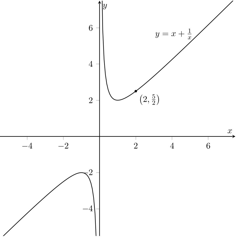
_images/x%2B1%2Cx.png — Fig. 6.6 Graph of $y=x+ \frac{1}{x}$, and the point $\left(2,\frac{5}{2}\right)$.#

Solution.
We first find the equation of tangent at the point $(2,\frac 52)$. Let $f(x) = x + x^{-1}$. Then $f'(x) = 1-x^{-2}$. We are working at the point $(2,\frac{5}{2})$ so, putting $x=2$, we get

\[ f'(2)=1-2^{-2}=1-\frac{1}{4}=\frac{3}{4}. \]

Thus the tangent at the point $(2,\frac{5}{2})$ has equation

\[\begin{align*} y &= f'(2)x+c\\ &= \frac{3}{4}x+c \end{align*} \]

for some constant $c$. Since we require that $y=\frac{5}{2}$ when $x=2$ we get $\frac{5}{2}=\frac{3}{4}.2 + c$ so that $c=\frac{5}{2}-\frac{3}{2}=1$. Thus the tangent to the curve $y=f(x)$ at the point $(2,\frac{5}{2})$ is the line

\[ y=\frac{3}{4}x +1. \]

We now find the equation of the normal at the point $(2,\frac 52)$. We know that the normal is perpendicular to the tangent so, denoting its gradient by $m$ and using equation (6.4), we find that

\[ m \times \frac{3}{4}=-1. \]

Hence $m=-\frac{4}{3}$ and our line has equation $y=-\frac{4}{3}+d$ for some $d$. But the normal also has to pass through the point $(2,\frac{5}{2})$, so that $\frac{5}{2}=-\frac{4}{3}.2 + d$ and hence $d=\frac{5}{2}+\frac{8}{3}=\frac{31}{6}$. It follows that the equation of the normal at the point $(2,\frac{5}{2})$ is

\[ y=-\frac{4}{3}x + \frac{31}{6} \]

(or, we could write that the equation of the normal is $n(x)=-\frac{4}{3}x + \frac{31}{6}$).

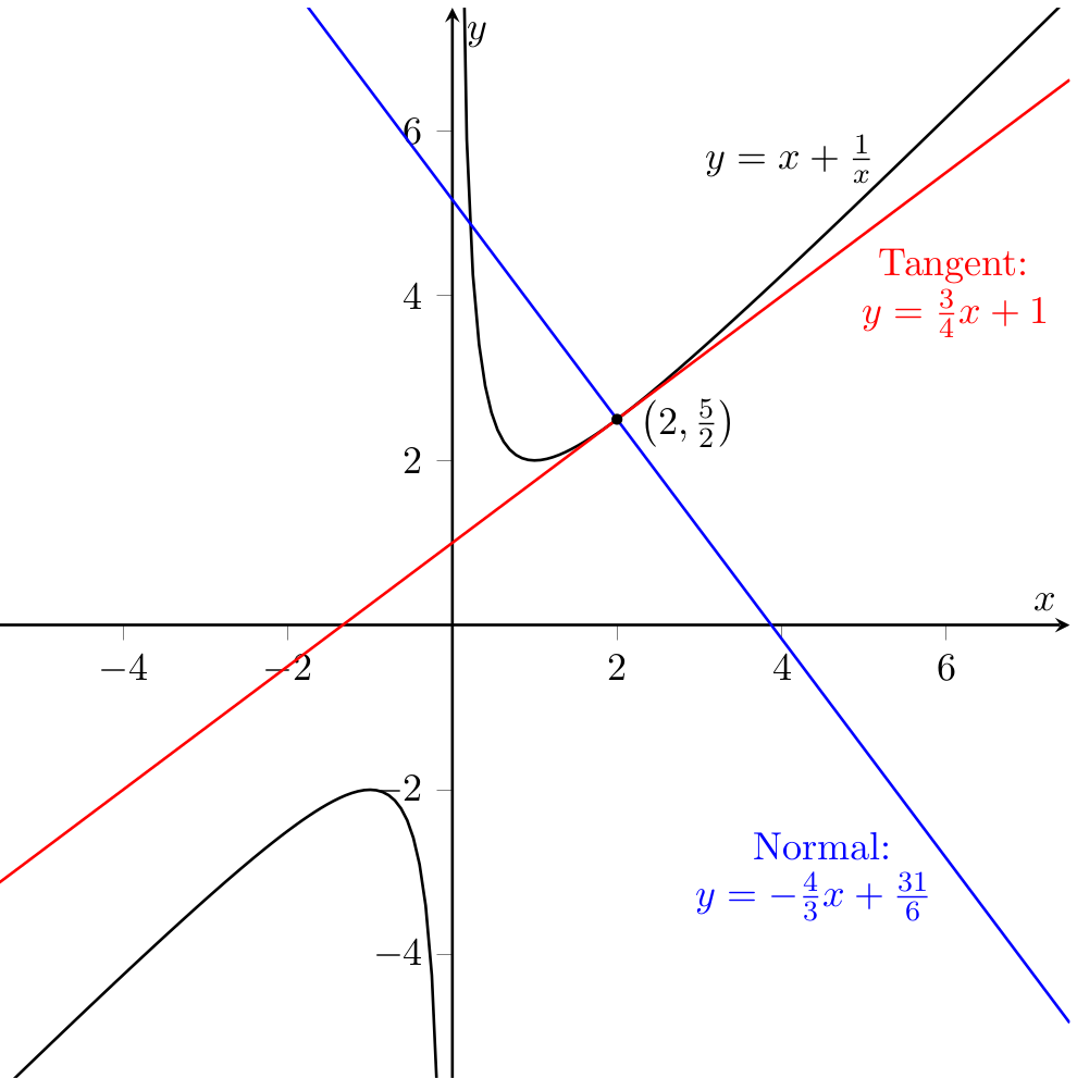
_images/x%2B1%2Cxtangentnormal.png — Fig. 6.7 The tangent and normal to $y=x+ \frac{1}{x}$ at $\left(2,\frac{5}{2}\right)$.#

Applications
As well as providing good differentiation practice, tangents and normals are used frequently in applications. For example, if a particle is moving along a given trajectory, its velocity always points along a tangent line to its position, and acceleration acceleration points along a normal line.

6.5. Small Changes#

Let $y=f(x)$ and consider a point $P=(a,f(a))$ on the curve. Now, suppose we make a small change in $x$, say $x$ changes from $a$ to $a + \delta x$ for some small number $\delta x$. Then there will be an associated change in $y$, say $y$ changes from $f(a)$ to $f(a)+ \delta y$ for some small number $\delta y$. If $Q$ is the point $(a + \delta x, f(a)+\delta y)$ (our point after $x$ has changed a little) then the gradient of the line $PQ$ is $\frac{f(a)+\delta y -f(a)}{a+\delta x-a}=\frac{\delta y}{\delta x}$ and, as $\delta x \rightarrow 0$, this tends to the value of $\frac{dy}{dx}$ at $a$ (written $\left.\frac{dy}{dx}\right|_{x=a}$) by the first principle of differentiation. So,if $\delta x$ is small (that is, very near to 0) then $\frac{\delta x}{\delta y}\approx\left.\frac{dy}{dx}\right|_{x=a}$ and thus, multiplying both up by $\delta x$, $\delta y \approx \left.\frac{dy}{dx}\right|_{x=a} \delta x$.

Hence, given a small change in $x$ at the point $P=(a,f(a))$ we have found the formula

Change in $\displaystyle y \approx \left.\frac{dy}{dx}\right|_{x=a} \times$(small change in $x$).

Note

In the above formula, $\frac{dy}{dx}$ is evaluated at the point $P=(a,f(a))$ we started with. If, for example, $y=x^2$ and $P=(2,4)$, then $\frac{dy}{dx}=2x$ and our formula for small changes at $P$ gives

\[\begin{align*} \mbox{change in } y &\approx \left.\frac{dy}{dx}\right|_{x=2}\times (\mbox{small change in $x$})\\ &= \left.(2x)\right|_{x=2}\times (\mbox{small change in $x$})\\ &= 4\times (\mbox{small change in $x$}) \end{align*}\]

Example 6.13

Using the method of small changes, find the approximate increase (in $\mbox{mm}^3$) of the volume of a cube whose side increases from $10$ to $10.2$mm.

Solution.
Let $x$ be the length of a side in mm and $V$ be the volume of the cube in $\mbox{mm}^3$. Then $V = x^3$ and so $\frac{dV}{dx} = 3x^2$. Hence we get $\left.\frac{dV}{dx}\right|_{x=10} = 3\times 10^2 = 300$. So the change in the volume is approximately

\[ \left.\frac{dV}{dx}\right|_{x=10}\times\mbox{(small change in $x$)} = 300\times 0.2 = 60, \]

that is the volume change is approximately $60\mbox{mm}^3$.

Note that the actual change can be calculated directly as $(10.2)^3 - 10^3 = 61.208$mm which is pretty close to what we found.

Example 6.14

Find the approximate percentage increase in the area of a circle whose radius is increased by $2\%$.

Solution.
The area $A$ of a circle of radius $r$, whatever the units, is given by $A = \pi r^2$ so $\frac{dA}{dr} = 2\pi r$. If the radius at the start is $r_0$, we are given that the radius increases by $2\%$, that is the small change in $r$ is $\frac{2}{100}\times r_0$. Thus, using the formula for small changes, we get

\[\begin{align*} \text{Change in }A &\approx \left.\frac{dA}{dr}\right|_{r=r_0}\times (\text{small change in }r) \\ &= 2\pi r_0 \times \frac 2{100} r_0\\ &= \frac{4\pi r_0^2}{100}. \end{align*}\]

Since the percentage change in $A$ is given by

\[ \frac{\mbox{change in $A$}}{\mbox{$A$}}\times 100 \% \]

we get

\[\begin{align*} \mbox{Percentage change in $A$} &\approx \frac {4\pi r_0^2}{100}.\frac{1}{\pi r_0^2} \times 100\%\\ &= 4\%. \end{align*}\]

So the area increases by approximately $4\%$.

6.6. Second and Higher Derivatives#

Mathematicians have a sort of rule: if it works once, why not try it again? This leads to the concept of higher derivatives. Given a function $y=f(x)$ we know that we can differentiate it to obtain $\frac{dy}{dx}$. But this is again a function of $x$. Hence we can differentiate again — and again. We make the following definitions.

Definition 6.5

The second derivative of $y=f(x)$ is the result of differentiating twice. We write

\[ \frac{d^2y}{dx^2} = f''(x) = \frac{d}{dx}\left(\frac{dy}{dx}\right). \]

The third derivative of $y=f(x)$ is the result of differentiating three times. We write

\[ \frac{d^3y}{dx^3} = f'''(x) = \frac{d}{dx}\left(\frac{d}{dx}\left(\frac{dy}{dx}\right)\right). \]

More generally, if $n$ is a positive integer, then the $n^{\text{th}}$ derivative of $y=f(x)$ is the result of differentiating $n$ times.

We write

\[ \frac{d^ny}{dx^n} = f^{(n)}(x) = \underbrace{\frac{d}{dx}\Bigg(\ldots\frac{d}{dx}\Bigg(\frac{dy}{dx}}_{n\text{ times}}\Bigg)\ldots\Bigg) \]

Example 6.15

Let $y = f(x) = x^2 - 3\sqrt{x} +2$. Then $\displaystyle\frac{dy}{dx} = 2x - \frac{3}{2}x^{-\frac{1}{2}}$, so

\[ \frac{d^2y}{dx^2}=f''(x) = 2+\frac{3}{4}x^{-\frac{3}{2}}, \hspace{3em} \frac{d^3y}{dx^3}=f'''(x) = -\frac{9}{8}x^{-\frac{5}{2}}, \]

\[ \frac{d^4y}{dx^4}=f^{(4)}(x) = \frac{45}{16}x^{-\frac{7}{2}}, \hspace{3em} \frac{d^5y}{dx^5}=f^{(5)}(x) = -\frac{315}{32}x^{-\frac{9}{2}}, \]

and so on.

Note the switch in notation from repeated dashes to numbers in brackets. It is standard practice to do this from about the fourth derivative onwards, as too many dashes in a row gets confusing to look at.

The second derivative, $\frac{d^2y}{dx^2}$ or $f''(x)$, crops up in many circumstances. Revisiting an example from earlier in the course, if $y$ represents distance and $x$ is time, then $\frac{dy}{dx}$ is speed (or velocity) and $\frac{d^2y}{dx^2}$ is acceleration. Next chapter, we will sometimes use it to determine the nature of stationary points.

Differentiation

Contents

6. Differentiation#

6.1. Tangents and Gradients#

6.1.1. Approximation Method I#

6.2. Approximation Method II#

6.2.1. Precise Method — First Principles Differentiation#

6.3. Differentiation#

6.4. Tangents and Normals#

6.5. Small Changes#

6.6. Second and Higher Derivatives#