7. Stationary Points#
Consider Fig. 7.1 and Fig. 7.2 below.
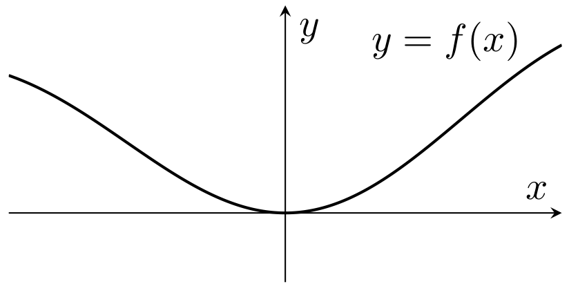
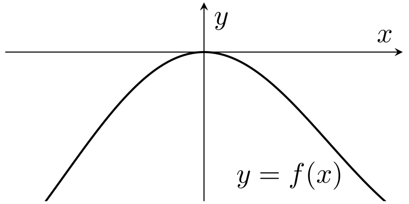
Both show what are known as turning points: Fig. 7.1 shows an example of a local minimum at \(x=0\) and Fig. 7.2 shows an example of a local maximum, again at \(x=0\). Note that in each case, at the turning point the tangent to the curve is horizontal.
Now have a look at Fig. 7.3 and Fig. 7.4.
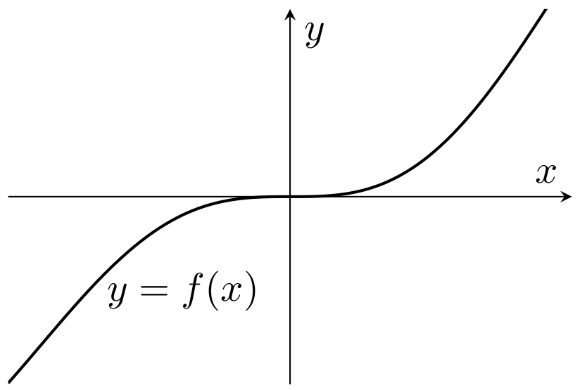
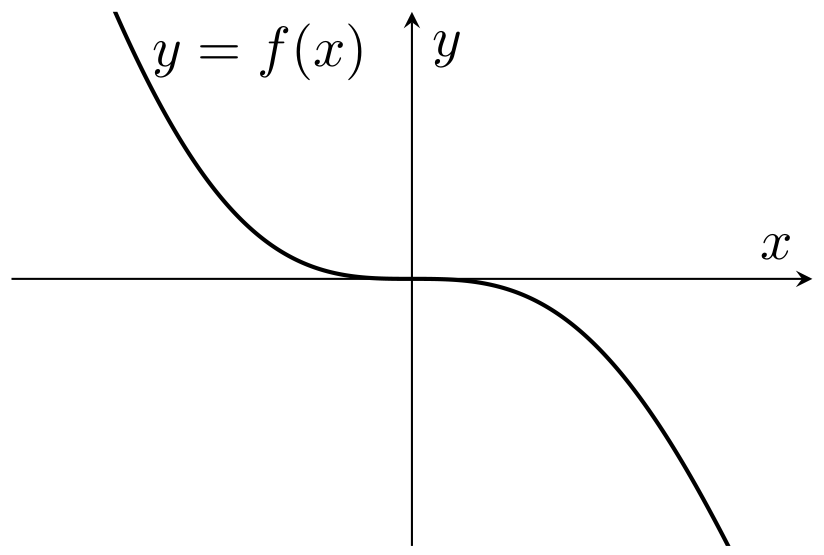
Here, when \(x=0\), we again find that the tangent line is horizontal but this time we have neither a maximum or a minimum. These are examples of a point of inflection.
We make the following definition.
Definition 7.1
On a curve \(y=f(x)\), points where \(\frac{dy}{dx} = 0\) are called stationary points. They come in three types: local maxima, local minima and points of inflection.
7.1. Identifying and Classifying Stationary Points#
We can find the location of the stationary points of a curve \(y=f(x)\), by differentiating and solving \(f'(x)=0\) for \(x\).
In this section we do this, and we also look at two (related) methods for classifying stationary points: the L-R table, and the second derivative test.
7.1.1. Method I: The L-R Table#
Looking at Fig. 7.1, Fig. 7.2, Fig. 7.3 and Fig. 7.4 once more, notice that
For a \textbf{local minimum}, the gradient \(\frac{dy}{dx}\) begins negative, then is zero, then is positive, as \(x\) increases.
For a \textbf{local maximum}, we see that \(\frac{dy}{dx}\) goes from positive, to zero and then to negative.
For a \textbf{point of inflection}, \(\frac{dy}{dx}\) does not change sign — it is either positive, then zero, then positive again, or negative, then zero, then negative.
Hence, we have a method for finding and identifying stationary points: first find the points at which \(\frac{dy}{dx} = 0\), and then look at how \(\frac{dy}{dx}\) behaves just to either side of these points.
Example 7.1
Find the stationary points of \(y = 2x^3 + 3x^2 - 12x +1\) and determine their nature.
Solution.
We first differentiate \(y\) and find the stationary points by seeing where \(\frac{dy}{dx} = 0\).
Thus \(\frac{dy}{dx} = 0\) at \(x=1\) and \(x=-2\). When \(x=1\) we get \(y=2\times 1^3 + 3\times 1^2 -12\times 1 + 1 = -6\). When \(x = -2\) we get \(y=2\times (-2)^3 + 3\times (-2)^2 -12\times (-2) + 1 = 21\). Hence, the stationary points are \((1,-6)\) and \((-2,21)\).
To determine the nature of the stationary points, we need to look at \(\frac{dy}{dx}\) first near to \(x= 1\) and then near to \( x= -2\). To make things easier, we write \(SP\) for stationary point, \(L\) for a point which is slightly to the left of the stationary point and \(R\) for a point which is slightly to the right of the stationary point.
Warning
We have to make sure here that we choose points \(R\) and \(L\) so that the only stationary point between them is the one we already know about.
For the stationary point at \(x = 1\) we get the following table.
\(L\) |
\(SP\) |
\(R\) |
|
|---|---|---|---|
\(x\) |
\(0\) |
\(1\) |
\(2\) |
\(\frac{dy}{dx}\) |
\(-12\) |
\(0\) |
\(6\times 1\times 4\) |
Gradient |
\(-\)ive |
\(0\) |
\(+\)ive |
Similarly, at \(x=-2\) we have
\(L\) |
\(SP\) |
\(R\) |
|
|---|---|---|---|
\(x\) |
\(-3\) |
\(-2\) |
\(0\) |
\(\frac{dy}{dx}\) |
\(24\) |
\(0\) |
\(-12\) |
Gradient |
\(-\)ive |
\(0\) |
\(+\)ive |
So when \(x = 1\) we have a local minimum (that is \((1, -6)\) is a local minimum) and when \(x = -2\) we have a local maximum (that is \((-2,21)\) is a local maximum).
Remark 7.1
To remember which type of stationary point corresponds to which pattern of gradient changes, it may be helpful to draw under the tables, as illustrated below.
\(L\) |
\(SP\) |
\(R\) |
|
|---|---|---|---|
Gradient |
\(-\)ive |
\(0\) |
\(+\)ive |
Picture |
\(\diagdown\) |
\(\_\_\_\) |
\(\diagup\) |
Here we notice that we are looking at a local minimum.
We summarise the workflow for finding and identifying stationary points below.
Method I for finding stationary points To find the stationary points on the curve \(y = f(x)\)
Find \(\frac{dy}{dx}\).
Solve \(\frac{dy}{dx} = 0\).
Make an \(L-R\) table for each stationary point.
(Make sure that \(L\) and \(R\) straddle just one stationary point.)
Example 7.2
Find the stationary points of \(y = f(x) = x^3(x-1)^2 \) and determine their nature.
Solution.
Until we have some more rules to deal with a function of this type, we have to multiply out the brackets to get \(y = f(x) = x^5 -2x^4 +x^3\). Now \(\frac{dy}{dx} = f'(x) = 5x^4 -8x^3+3x^2 = x^2(5x^2 -8x +3) = x^2(x-1)(5x-3)\). Thus we have three SPs, \(P_0 = (0,0)\), \(P_1 = \left(\frac 35, \frac{108}{3125}\right)\) and \(P_2 = (1,0)\).
I here combine all the three SPs into one table to ensure that I separate my SPs properly:
\(L\) |
\(SP_0\) |
\(M_1\) |
\(P_1\) |
\(M_2\) |
\(P_2\) |
\(R\) |
|
|---|---|---|---|---|---|---|---|
\(x\) |
\(-1\) |
\(0\) |
\(\frac 12\) |
\(\frac 35\) |
\(\frac 34\) |
\(1\) |
\(2\) |
\(f'(x)\) |
\(>0\) |
\(0\) |
\(>0\) |
\(0\) |
\(<0\) |
\(0\) |
\(>0\) |
Shape |
\(\diagup\) |
\(\_\_\_\) |
\(\diagup\) |
\(\_\_\_\) |
\(\diagdown\) |
\(\_\_\_\) |
\(\diagup\) |
Thus \(P_0 = (0,0)\) is a point of inflection, \(P_1 = \left(\frac 35, \frac{108}{3125}\right)\) is a local maximum and \(P_2 = (1,0)\) is a local minimum.
Remark 7.2
Most mistakes happen because of not choosing the right points to separate the SPs. Whenever you choose points, you need to ensure that the only have exactly one SP between them. You also have to ensure that if the graph of function splits into different parts (due to holes in domain), you keep in the part where your SP is.
Example 7.3
Find the SPs of \(f(x) = x + \frac 1x\) and determine their nature.
Solution.
Note that the function has domain \(\{ x\in \mathbb{R}\::\: x \neq 0\}\).
We find that \(f'(x) = 1 - \frac 1{x^2}\) and to find the SPs, we solve \(1 - \frac 1 {x^2} = 0\) for \(x \neq 0\). We get that \(x^2 = 1\) and so the SPs are at \(P = (-1,-2)\) and \(Q = (1,2)\).
For \(P\), we need to choose points left and right from \(-1\) which lie on the left hand side of the graph, i.e.~are less than zero.
\(L\) |
\(SP\) |
\(R\) |
|
|---|---|---|---|
\(x\) |
\(-2\) |
\(-1\) |
\(-\frac{1}{2}\) |
\(f'(x)=1-\frac{1}{x^2}\) |
\(+\)ive |
\(0\) |
\(-\)ive |
means that \(P = (-1,-2)\) is a local maximum.
For \(Q\), we need to choose points left and right from \(1\) which lie on the right hand side of the graph, i.e.~are greater than zero.
| | \(L\) |\(SP\)| \(R\) | | \(x\) |\(\frac 12\)|\(1\) | \(2\) | |\(f'(x)=1-\frac{1}{x^2}\) | \(+\)ive | 0 |\(-\)ive|
means that \(Q = (1,2)\) is a local minimum.
I leave it to you to mess the points up and see what happens!
7.1.2. Method II: The Second Derivative Test#
What does \(\frac{d^2y}{dx^2}\) measure? The answer is it tells us how \(\frac{dy}{dx}\) (and hence the gradient of the curve \(y=f(x)\)) changes with \(x\). If \(\frac{d^2y}{dx^2}\) is positive at a particular point, then we know the gradient of \(y=f(x)\) is increasing as \(x\) increases through that point. If \(\frac{d^2y}{dx^2}\) is negative at a particular point, then we know the gradient of \(y=f(x)\) is decreasing as \(x\) increases through that point. However, if \(\frac{d^2y}{dx^2}\) is zero at a particular point the deduction is that the gradient is changing very slowly around that point — how it is changing, we can’t tell.
The above ideas give us an alternative method for identifying stationary points.
Example 7.4
Find the stationary points of \(y = 5x^6 - 18x^5 + 15 x^4\) and determine their nature.
Solution.
We begin by differentiating.
Hence \(\frac{dy}{dx} = 0\) if and only if \(x = 0\), \(x = 1\) or \(x = 2\). Thus the stationary points are \((0,0)\), \((1,2)\) and \((2,-16)\).
We next find the second derivative.
When \(x = 1\) we get \(\frac{d^2y}{dx^2} = 30\times(-1)\) which is negative. Hence, the gradient is decreasing as we pass through \(x=1\). Since the gradient is zero at our stationary point, to the left of it the gradient must be positive and to the right negative. Hence, we have a local maximum at \((1,2)\).
When \(x = 2\) we get \(\frac{d^2y}{dx^2} = 30(4)(20-24+6)\) which is positive. In this case the gradient is increasing as we pass through \(x=2\), so it must be negative to the left and positive to the right. Thus we have a local minimum at \((2,-16)\).
When \(x = 0\) we get \(\frac{d^2y}{dx^2} = 0\). This is the least helpful outcome: it means that we have to use Method I to determine the nature of this stationary point. Note our choice of right hand (R) point below has to be less than 1, since there is another stationary point there.
\(L\) |
\(SP\) |
\(R\) |
|
|---|---|---|---|
\(x\) |
\(-1\) |
\(0\) |
\(\frac{1}{2}\) |
\(\frac{dy}{dx}\) |
\(-30(-2)(-3)\) |
\(0\) |
\(30(0.5)^3(-1.5)(-0.5)\) |
Gradient |
\(-\)ive |
\(0\) |
\(+\)ive |
Hence we have a local minimum at \((0,0)\).
We summarise the workflow that we used above.
Summary: Method II for finding stationary points
To find stationary points on the curve \(y = f(x)\)
Find \(\frac{dy}{dx}\) and \(\frac{d^2y}{dx^2}\).
Solve \(\frac{dy}{dx} = 0\).
At each stationary point, if \(\frac{d^2y}{dx^2}\) is positive then we have a local minimum, if \(\frac{d^2y}{dx^2}\) is negative we have a local maximum, and if \(\frac{d^2y}{dx^2} = 0\) we use an \(L-R\) table to determine its nature.
Example 7.5
Example 7.3 revisted.
The function \(y = f(x) = x + \frac 1{x}\) has domain \(\{ x \in \mathbb{R}\::\: x \neq 0\}\) and two SPs, namely \(P= (-1,-2)\) and \(Q = (1,2)\). Because of the hole in the domain, we had to be especially careful when selection our points for the L-R-table. So using the second method is much easier here.
We have \(y" = f''(x) = \frac{2}{x^3}\). Now \(f''(-1) < 0\) so \((-1,-2)\) is a local maximum; and \(f''(1) > 0\) so that \((1,2)\) is a local minimum.
7.2. Sketching Graphs#
So far in the first term, we looked at the graphs of standard functions and shifts and stretches of them. For general functions, we need and have a different function.
The idea for sketching graphs, whether a standard function or not, is to use key features, such as stationary points, along with the overall behaviour of the function to get a picture of its graph. This is much more reliable than making a table and plotting points! If you are asked to sketch a graph, you need to use either the methods of the first term or the method we illustrate a method below. Note that plotting will not give you marks in the exam.
7.2.1. Graphs of functions with domain \(\mathbb{R}\)#
At the moment, the only functions we have are polynomial functions for this section, but the flow works for all functions with domain \(\mathbb{R}\), that is functions where there are no restrictions on the domain. If the question tells you to restrict the domain, you can still follow this flow and then redraw the graph with your restricted domain as we did last term.
Example 7.6
Sketch the graph of \(y = 3x^5 - 5x^3\).
Solution.
We work through the following steps.
This function has domain \(\mathbb{R}\). That is, it is defined for any real number — there are no values of \(x\) that must be avoided.
Where possible, we determine where the function crosses the \(x\)-axis (that is, we solve \(f(x) = 0\)) and where the graph crosses the \(y\)-axis (that is, evaluate \(f(0)\)).
Now \(f(x) = x^3(3x^2 -5)\) so that the graph crosses the \(x\)-axis at \(x = 0\), \(x = \sqrt{\frac 53}\) and \(x = - \sqrt{\frac{5}{3}}\). As we are making a sketch, it will be helpful to get an approximate value of \(\sqrt{\frac 53} \approx 1.3\). Clearly, \(f(0) = 0\) so the graph crosses the \(y\)-axis at \(0\).Next, we find the stationary points and determine their nature. \begin{align*} \frac{dy}{dx} &= 15x^4 - 15x^2\ &= 15x^2(x^2-1)\ &= 15x^2(x-1)(x+1)\ \mbox{and}\quad\frac{d^2y}{dx^2} &= 60x^3 - 30 x\ &= 30x(2x^2-1). \end{align*} Thus the stationary points are \(P_1=(-1,2)\), \(P_2=(0,0)\) and \(P_3=(1,-2)\).
When \(x=-1\), \(\frac{d^2y}{dx^2} = -30<0\) so \(P_1\) is a local maximum.
When \(x=1\), \(\frac{d^2y}{dx^2} = 30>0\) so \(P_3\) is a local minimum.
When \(x=0\), \(\frac{d^2y}{dx^2} = 0\) so we need an LR table.
| | \(L\) | \(P_2\) | \(R\) | | \(x\) |\(-0.5\) | \(0\) | \(0.5\) | |\(\frac{dy}{dx}\) | \(-\frac{45}{16}\) | \(0\) | \(-\frac{45}{16}\)| | Gradient |\(-\)ive | \(0\) | \(-\)ive |
So \(P_2\) is a point of inflection.
We next consider the behaviour as \(x \rightarrow \pm \infty\).
As \(x \rightarrow +\infty\) (that is, as \(x\) gets bigger and bigger in the positive direction) we find that \( y \rightarrow +\infty\). This is because, for a polynomial function, we only need to look at the dominant term, that is the one with the highest exponent. In our case this is \(3x^5\) which will be positive and very large the bigger we choose \(x\).
(As an example, when \(x=10^{10}\), \(3x^5=3(10^{10})^5 = 3(10^{50})\) which is much bigger than \(5(10^{10})^3=5(10^{30})\); indeed the leading term has 20 more zeros on the end!)
As \(x \rightarrow - \infty\) we find that \( y \rightarrow - \infty\). This is again due to the dominant term \(3x^5\) which will get very large and negative if \(x\) is large and negative.Finally, we can draw the graph!
We choose a scale according to the key points we found. Mark the key points found in 1, 2 and 3 and join them with a smooth curve taking into account the behaviour identified in 4.
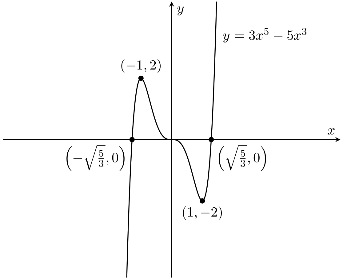
Fig. 7.5 The graph of \(y=3x^5-5x^3\), with stationary points and axis crossings marked.#
7.2.2. Sketches of graphs with vertical asymptotes#
A graph can have strange behaviour that might be missed in just plotting tabulated values. An example of when this can occur is with graphs involving reciprocals, such as \(\frac{1}{x}\). Often we find vertical asymptotes. More generally, these problems occur when there are values for \(x\) for which the function is not defined. Let’s look at an example.
Example 7.7
Sketch \(y = f(x) = x+ \frac 1x\).
Solution.
We first check the domain of the function.
We see that \(f(x)\) is not defined for \(x = 0\). Thus the domain is \(\{x\in \mathbb{R}\mid x\neq 0\}\).We look at where the function crosses the \(x\)- and \(y\)-axes. Note that, for \(x\neq 0\), \begin{align*} y=0 & \mbox{ so } & x+ \frac 1x = 0\ & \mbox{ so } & x^2 + 1=0\ & \mbox{ so } & x^2=-1.\end{align*} But \(x^2\geq 0\) for all \(x\in \mathbb{R}\), so we see that we can never have \(y=0\) and the graph does not cross the \(x\)-axis.
It also does not cross the \(y\)-axis as it is not defined for \(x=0\).Find the stationary points and determine their nature.
We calculate that \(\displaystyle \frac{dy}{dx} = 1-\frac1{x^2}\) and \(\displaystyle \frac{d^2y}{dx^2} = \frac2{x^3}\).
Thus the stationary points are where \(x=\pm 1\), that is \((1,2)\) and \((-1, -2)\).
When \(x = -1\) we have \(\frac{d^2y}{dx^2} < 0\), so \((-1,-2)\) is a local maximum.
When \(x = 1\) we have \(\frac{d^2y}{dx^2} > 0\), so \((1,2)\) is a local minimum.Consider what happens for \(x \rightarrow \pm \infty\). If \(x\) get very large, either positive or negative, \(\frac 1x \rightarrow 0\). Thus the \(x\) term is the dominate term. So, as \(x \rightarrow \infty\) we have \(f(x) \rightarrow \infty\) and as \(x \rightarrow - \infty\) we have \(f(x) \rightarrow - \infty\).
Consider what happens around the point where \(f(x)\) isnot defined.
When \(x \rightarrow 0^-\), that is, when \(x\) is very small and negative, \(\frac 1x \rightarrow -\infty\) and so \(f(x) \rightarrow - \infty\) for \(x \rightarrow 0^-\).
When \(x \rightarrow 0^+\), that is, when \(x\) is very small and positive, \(\frac 1x \rightarrow \infty\) and so \(f(x) \rightarrow \infty\) for \(x \rightarrow 0^+\).Draw the sketch:
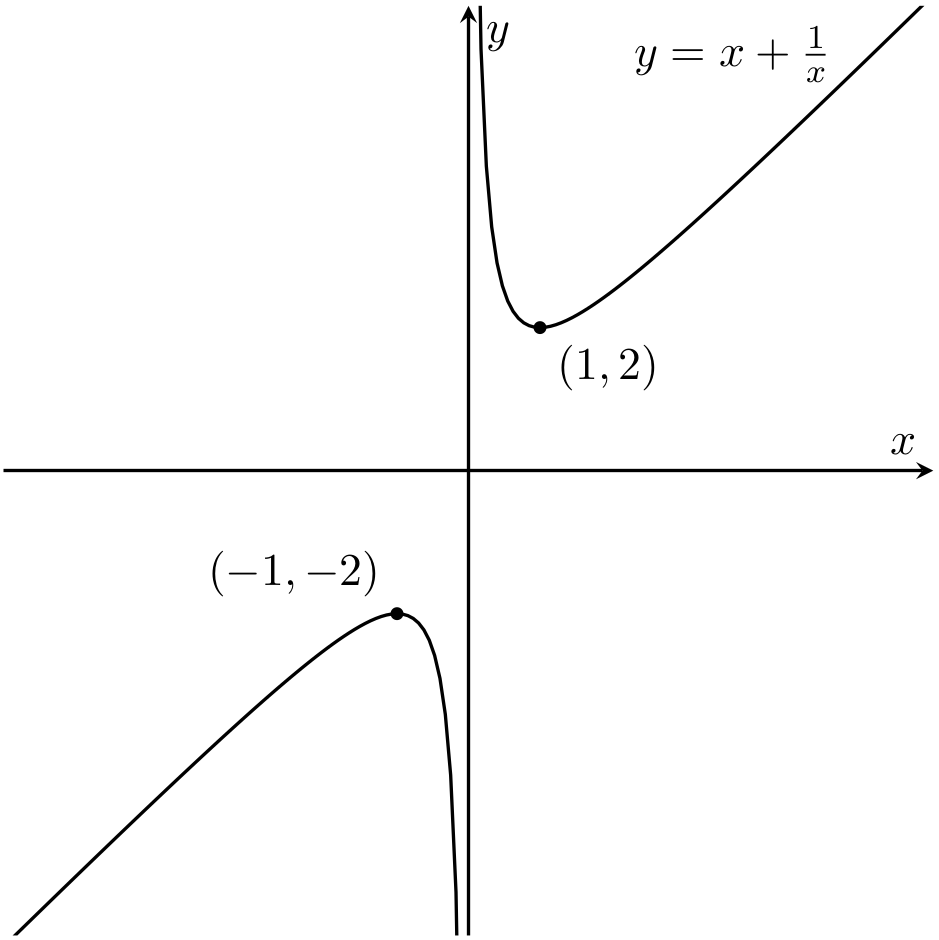
Fig. 7.6 The stationary points of \(y=x+ \frac{1}{x}\).#
The behaviour at \(x = 0\) is an example of a vertical asymptote.
Here is a list of the asymptotical behaviour of \(x^n\) for \(n > 0\):
For \(x \rightarrow \infty\), we have:
\(x^n \rightarrow \infty\) as \(x \rightarrow \infty\);
\(x^n \rightarrow -\infty\) as \(x \rightarrow \infty\);
\(x^{-n} \rightarrow 0\) as \(x \rightarrow \infty\);
\(x^{-n} \rightarrow 0\) as \(x \rightarrow \infty\).
For \(x \rightarrow - \infty\), we need to check whether the exponent is odd or even and get
\(x^{2n-1} \rightarrow -\infty\) as \(x \rightarrow -\infty\);
\(x^{2n} \rightarrow \infty\) as \(x \rightarrow -\infty\);
\(x^{2n-1} \rightarrow \infty\) as \(x \rightarrow -\infty\);
\(x^{2n} \rightarrow -\infty\) as \(x \rightarrow -\infty\);
\(x^{-n} \rightarrow 0\) as \(x \rightarrow -\infty\);
\(x^{-n} \rightarrow 0\) as \(x \rightarrow -\infty\).
For \(x \rightarrow 0^+\) we get
\(x^{-n} \rightarrow \infty\) as \(x \rightarrow 0^+\);
\(x^{-n} \rightarrow -\infty\) as \(x \rightarrow 0^+\).
And finally for \(x \rightarrow 0^-\) we again have to check whether the exponent is odd or even and get
\(x^{-2n+1} \rightarrow -\infty\) as \(x \rightarrow 0^-\);
\(x^{-2n} \rightarrow \infty\) as \(x \rightarrow 0^-\);
\(x^{-2n+1} \rightarrow \infty\) as \(x \rightarrow 0^-\);
\(x^{-2n} \rightarrow -\infty\) as \(x \rightarrow 0^-\).
7.3. Applications of Maxima and Minima to Problems#
Let’s look at some examples of how we can apply the theory we have developed so far.
Example 7.8
A closed cylindrical can has a volume \(128\pi\mbox{m}^3\). What is the minimum possible surface area of the can?
Solution.
Let \(r\) be the radius of the can and \(h\) be its height. We start by writing down the relevant formulae. Recall that the volume of a cylinder is given by \(V= \pi r^2h\) and the surface area of a cylinder is \(A = 2\pi r^2 +2\pi rh\) (each end section has area \(\pi r^2\) and the curved surface has area \(2\pi r h\)).
As the volume of the can is \(128\pi\) we have \(128\pi = \pi r^2h\) so that \(h = \frac{128}{r^2}\). Note that \(r\) (that is, the radius of the cylinder) must be positive, so in particular \(r\neq 0\). Substituting our expression for \(h\) into the equation for the area we get
Now \(\frac{dA}{dr} = 2\pi\left(2r - \frac{128}{r^2}\right)\) and \(\frac{d^2A}{dr^2} = 2\pi\left(2+\frac{256}{r^3}\right)\). We find the stationary points for this function by solving \(\frac{dA}{dr}=0\).
Thus we have one stationary point, ocurring when \(r =4\). At \(r=4\) we find \(\frac{d^2A}{dr^2} = 2\pi(2+ \frac{256}{4^3})>0\) so this is a local minimum.
Thus the minimum value for the area \(A\) is when \(r = 4\) and thus the minimum surface area is
Note that the height of the can will be \(h = \frac{128}{r^2} = \frac{128}{4^2} = 8\).
Example 7.9
A rectangular box is to be sent by an airline whose regulations say that the base of the box must be square and the sum of the three dimensions must be no more than 6 metres. What is the maximum volume that can be obtained?
Solution.
Let \(x\) be the length of the side of the base, in metres. As the sum of the three dimensions of the box must not be more than 6 metres, the maximum height the box can have is \(6-2x\) (clearly, the higher the better). The volume of the box is then
(in metres cubed).
We find that \(\frac{dV}{dx} = 12 x - 6x^2 = 6x(2-x)\) and \(\frac{d^2V}{dx^2} = 12 - 12x\). Thus the stationary points are when \(x = 0\) and \(x = 2\). When \(x = 0\) we definitely have a local minimum (we can see this since \(\frac{d^2 V}{dx^2} = 12>0\) when \(x=0\)), as should be expected! When \(x = 2\) we get \(\frac{d^2 V}{dx^2} = 12-24 = -12 < 0\), so this is a local maximum. Thus the biggest volume possible is when \(x = 2\), that is the maximum volume is \(V = 4(6-4)= 8\) metres cubed.