---

Chapter 2: Magnitudes

An astrononomy quirk - magnitudes

Generally speaking the flux is a perfectly useful measure of how much light we receive on Earth. There are some practical difficulties in measuring the flux of course; our detectors are not 100% efficient, and we have to correct for the amount of light absorbed by the atmosphere. Nevertheless, once these corrections have been made, there should be no problem reporting the amount of light received as fluxes, right? However, astronomy is a science with a tendency towards unconventional units of measure, and no exception is made here.

In astronomy, we often use the apparent magnitude instead of the flux. The scale upon which magnitude is now measured has its origin in the ancient Greek practice of dividing those stars visible to the naked eye into six magnitudes. The brightest stars were said to be of first magnitude (m = 1), while the faintest were of sixth magnitude (m = 6), the limit of human visual perception (without the aid of a telescope). Each grade of magnitude was considered to be twice the brightness of the following grade (a logarithmic scale). Nowadays, magnitude is still a logarithmic scale, but has been put on a formal footing. The apparent magnitude is related to the monochromatic flux by

(4)\[m_\nu = -2.5 \log_{10} F_{\nu} + c.\]

However, the ancient Greek convention has been retained; brighter stars have smaller magnitudes than fainter ones - courtesy of that minus sign in equation (4). So a star with magnitude -3 is much brighter than a star of magnitude 14. What is the value of the constant, \(c\) in equation (4)? In fact, we are free to choose any value we like, as long as we keep the same value between measurements. Although magnitudes can be a bit confusing on first acquaintance, they have one big advantage; the numbers involved tend to be easy to deal with. A magnitude of 0 is a lot quicker to grasp and remember than a flux of \(3.44\times10^{-8}\) W m^-2 μm^-1!

Measuring magnitude: Photometry

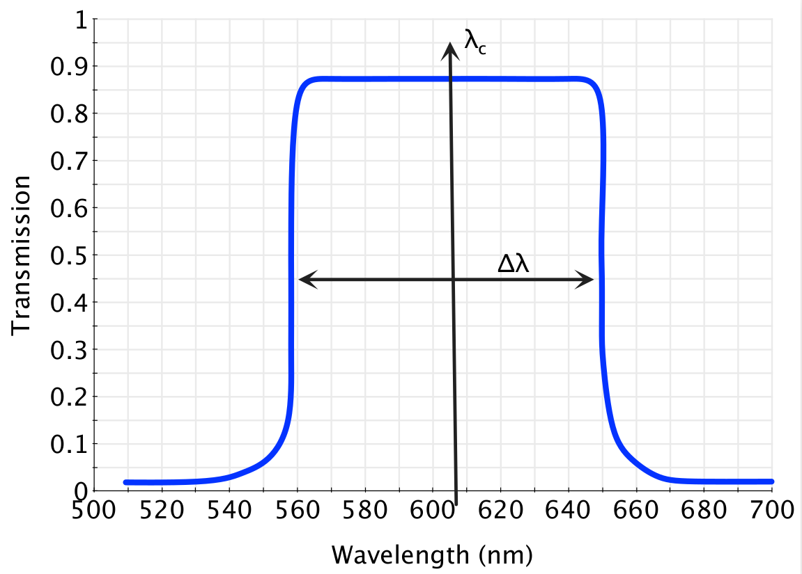
Fig. 8 Astronomical filter

Johnson Cousins filters

The technique of measuring accurate fluxes and magnitudes of astronomical sources is called photometry. Photometric systems are defined by the sets of filters which are used to isolate individual wavelength ranges in order to measure a monochromatic flux. An example filter set is shown in figure 8. This is the Johnson-Cousins filter set, which is widely used throughout astronomy, where \(U\), \(B\), \(V\), \(R\) and \(I\) refer to ultraviolet, blue, visual, red and infrared light. These are extended to longer IR wavelengths with the rather unimaginatively named \(J\), \(H\) and \(K\) set of filters.

In principle, astronomical photometry is simple. Consider the idealised filter shown in figure 8. This filter has a central (average) wavelength of \(\lambda_c\) and a width of \(\Delta \lambda\). This filter is placed on a camera on a telescope with collecting area \(\Delta A\). The camera is exposed to light for a time \(\Delta t\). Not every photon which falls on the telescope will be recorded. Suppose our camera/telescope combination detects a fraction, η of the photons which fall on the telescope (we say it has an efficiency of η). Therefore, if we detect \(N\) photons, the total number of photons which fell on our telescope was \(N/\eta\). What is the average energy of each of these photons? They have an average energy of \(E=h\nu = hc/\lambda\). So the total energy which arrived is

\(\Delta E = \frac{Nhc}{\eta \lambda}\).

The flux in our filter follows from

\(F_{\lambda} = \frac{\Delta E}{\Delta A \Delta t \Delta \lambda}\).

Fluxes in astronomical filters are normally referred to using the name of the filter as a subscript. As an example, the flux as measured in the Johnson V-band would be called \(F_V\). The V-band magnitude can be calculated in the usual way

\[m_V = -2.5 \log_{10} F_V +c_V .\]

Notice that I have called the constant \(c_V\), to indicate that this constant is specific to the V-band. In the Johnson photometric system, the constant \(c\) is chosen separately for each filter. The value of \(c\) is chosen so that the bright star, Vega (A0V), has a magnitude of zero in every band.

Magnitudes can be measured for a star in each photometric band and colour indices determined by subtracting the magnitudes as measured in different filters, e.g.

(5)\[\begin{split}\begin{align} m_B - m_V = B - V &= -2.5 \log_{10} F_B + c_B + 2.5 \log{10} F_V - c_V \\ &= +2.5 \log_{10} \frac{F_V}{F_B} + \text{const}. \end{align}\end{split}\]

Colour indices provide crude information about the spectra of astronomical sources (they are often just called the “colour”), and can be used to estimate the temperatures of stars. A couple of things are worth noting - because magnitudes are a logarithmic scale, subtracting two magnitudes is equivalent to dividing two fluxes. Also, since the magnitude scale is fixed so that the A star Vega has a magnitude of 0 in each band, Vega also has colour indices of zero, which fixes the constant in the equation above (\(F_{\rm V}/F_{\rm B}\) = 0.586 for Vega), so stars which are bluer than Vega possess a negative \(B-V\) index (or \(F_{\rm V}/F_{\rm B} <\) 0.586), and redder stars possess a positive \(B-V\) index (or \(F_{\rm V}/F_{\rm B} >\) 0.586). For reference, the Sun has \(B-V\) = +0.6 mag.

Absolute Magnitudes

We noted in the last section that the luminosity is a fundamental property of the source. The flux, by contrast, is a property both of the source, and its distance from us. The inverse square law tells us that a source can be faint (low in flux) because it is either intrinsically dim (low in luminosity), or very far away. Since the apparent magnitude is related to the flux, it too depends on the distance to the source. We would like a measure of intrinsic brightness for the magnitude scale; the magnitude equivalent of luminosity. This measure, which we will call the absolute magnitude, is the magnitude an object would have, if it were 10 parsecs away

Parsecs are a standard unit of distance in astrophysics. We’ll see why in the next section.

How are the absolute and apparent magnitude related? \(F_{\nu}\) is the flux of our object, and we’ll call the flux it would have at 10 parsecs \(F_{\nu}^{10}\). Let us measure the distance to our object, \(d\), in parsecs. The inverse square law tells us that

(6)\[\frac{F_{\nu}}{F_{\nu}^{10}} = \frac{L/4\pi d^2}{L/4\pi 10^2} = \left( \frac{10}{d} \right)^2.\]

Using equation (4) we can then write

\[\begin{split}\begin{align} M &= -2.5 \log_{10} F_{\nu}^{10} +c \text{, and} \\ m-M &= -2.5 \log_{10} F_{\nu} + 2.5 \log_{10} F_{\nu}^{10} \text{, or} \\ m-M &= -2.5 \log_{10} \left( \frac{F_{\nu}}{F_{\nu}^{10}} \right), \end{align}\end{split}\]

where M is the absolute magnitude. Combining this last equation with equation (6), we find

(7)\[m-M = 5 \log_{10} \left( \frac{d}{10} \right),\]

remembering all the while that \(d\) is measured in parsecs! Equation (7) tells us that the apparent and absolute magnitudes are related by the distance to the source; in fact, the quantity \(m-M\) is called the distance modulus. Distance moduli of \(m-M\) = 0, 5, 10, 15 mag therefore correspond to distances of 10, 100, 1000 and 10,000 parsec, respectively.

We can derive a general form of equation (7) too, which tells us how the apparent magnitude of an object changes with distance. We simply replace the 10 parsec distance we chose earlier by a general distance \(d_2\), and ask what it is the magnitude of our object at that distance \(m_2\)?

\[\begin{split}\begin{align} m-m_2 &= 5 \log_{10} \left( \frac{d}{d_2} \right) \text{, or} \\ m_1-m_2 &= 5 \log_{10} \left( \frac{d_1}{d_2} \right), \end{align}\end{split}\]

where I have replaced \(m\) and \(d\) with \(m_1\) and \(d_1\).

If we can measure the apparent magnitude for an object, and somehow know it’s absolute magnitude (perhaps all sources of a given type have the same absolute magnitude), then we can calculate the distance modulus, and from that, the distance. Generally speaking, however, we do not know the absolute magnitude of an object, and can only measure apparent magnitudes. How then, do we calculate the distance to astronomical objects? We will cover distance measurement in the next chapter.