
Chapter 6: Thermal Properties of Matter#
Up until now we’ve been focussing on the properties of radiation. We’ve seen that for an object where the radiation is in thermal equilibrium with the matter (a so-called black body), the spectrum of the radiation is given by the Planck curve, and we’ve looked at a few important properties of the Planck curve that allow us to obtain estimates of the temperature of stars.
Now I’d like to take a brief detour, and look at some of the properties of matter. In particular, we’re going to continue to study our idealised object in which thermal equilibrium between the matter and radiation is maintained. This has two very important consequences:
the radiation field and the matter have a well defined temperature and, since they are in thermal equilibrium with each other, the same temperature describes the radiation field and the matter
since the matter is in thermal equilibrium, it’s properties are described by the laws of statistical physics
Statistical physics is a way of looking at large systems. In a small-sized rooms, there might be something like air molecules. These molecules will be spread over a large range of speeds and energies. It is not possible in practice to calculate the behaviour of a single molecule in this room. Nevertheless, the gas in the room does have a few well defined properties, such as the pressure, temperature and density. Calculating these properties is the domain of statistical physics.
The idea behind statistical physics is although we cannot predict a single particle’s energy, or speed, what we can do is calculate the probability that it will have a given energy or speed. One of the most important results in statistical physics is that the probability of a particle having an energy, \(E\) depends upon the energy and temperature, like so
This is known as the Boltzmann distribution. The behaviour it predicts makes intuitive sense. The probability that a particle has energy, \(E\) depends on the energy and the temperature. At a given temperature, a particle is not likely to have energies much higher than \(kT\). Also, as the temperature increases, it becomes more likely that particles will have higher energies.
Deriving this equation is beyond us at the moment, but everything we will discuss today follows directly on from this result.
Maxwell-Boltzmann distribution of particle speeds#
Let’s consider our object in which the radiation and matter are in thermal equilibrium. Not every particle is going to have the same speed, so there will be a distribution of speeds. What is it? Amazingly, we can derive it using nothing more that the Boltzmann distribution. The details of the derivation involve some difficult maths, so I’m just going to cover the important steps below.
Since the gas in in thermal equilibrium, the Boltzmann distribution states that the probability that a gas particle has energy \(E\) is proportional to \(e^{-E/kT}\). But for a gas particle with speed \(v\) and mass \(m\), the energy is just the kinetic energy - \(E = \frac{mv^2}{2}\). So the probability that a particle as a speed \(v\), is given by
What we want to know is how many gas particles there are with speeds between \(v\) and \(v+dv\). Since \(dv\) is a very small change in speed, the probability that a particle has a speed in this range will simply be \(P(v)\), to a good approximation. The fraction of particles between \(v\) and \(v + dv\) is proportional to the probability a particle has this speed, multiplied by the number of possible speeds between \(v\) and \(v+dv\). The number of possible speeds turns out to be proportional to \(v^2 dv\). Finally, the total number of particles with speeds in the range of interest is the fraction of particles with these speeds multiplied by the total number of particles, \(n\), and so we can write that the number of gas particles with speeds between \(v\) and \(v+dv\) is
We can get rid of the proportionality by realising that if we integrate equation (15) over all speeds, the answer must equal the total number of particles, \(n\). Doing this gives the Maxwell-Boltzmann distribution of speeds in a gas:
This result gives the distribution of speeds in a gas which is in thermal equilibrium. The speeds of individual gas particles will change constantly as particles collide with each other, but the distribution of speeds within the gas as a whole does not change.
Properties of the Maxwell-Boltzmann distribution#
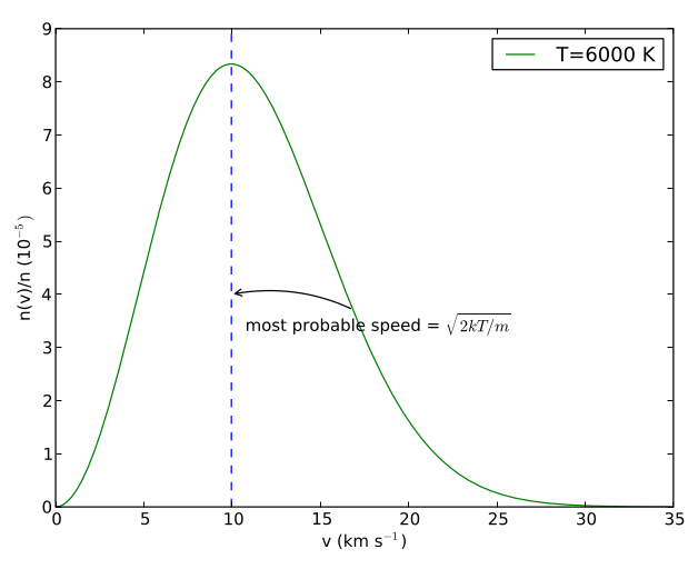
Fig. 27 Maxwell-Boltzmann distribution, \(n(v)/n\) for hydrogen atoms at a temperature of 6000 K, The most probable speed is labelled.#
Maxwell-Boltzmann distribution
What does the Maxwell-Boltzmann distribution look like? Figure 27 shows the distribution of speeds of hydrogen atoms at 6000K. At low speeds the \(v^2\) term in equation (16) dominates. Note that because of this there are no particles with zero speed, regardless of temperature! At high speeds, the exponential term dominates, which makes very high speeds (where \(mv^2 \gg 2kT\)) unlikely. In between there is a maximum of the Maxwell-Boltzmann distribution, which defines the most probable speed.
The most probable speed can be found by differentiating the Maxwell-Boltzmann distribution, and finding the point at which the slope is zero. Once again, the maths is awkward and adds nothing to our physical understanding, so I will just give the result, that the most probable (mode) speed is
The mean velocity is less straightforward to obtain, but it has a similar form:
Mean energy#
If we look again at figure 27, we see that it is not symmetric around the most probable speed. Instead, there is a tail extending towards higher velocities. What this means is that the mean of the distribution is not the same as the most probable speed (known as the mode of the distribution).
How do we calculate the mean speed or, more interestingly, the mean energy of the Maxwell-Boltzmann distribution? The mean energy is defined by
This equation should make sense to you; to calculate a mean you add up all the particle energies (\(\int n(E)\, E\, dE\)) and divide by the total number of particles, \(n\). We solve the integral in equation (17) by using \(E=\frac{1}{2} mv^2\) to convert the Maxwell-Boltzmann distribution into the distribution of energies, \(n(E)\). In doing so, we find the mean particle energy is
Since \(E=\frac{1}{2}mv^2\), we can determine the root-mean-squared velocity, which more accurately reflects the representative velocities than the mode or mean, reflecting better the high velocity tail of the Maxwell-Boltzmann distribution
Equipartition#
Before we move on to discuss the pressure of our gas, let’s take a quick look at our result for the mean energy. Our particles have a mean (kinetic) energy of \(\frac{3}{2} kT\). Of course, our particles are free to move in three dimensions, so their speed \(v\) has components directed along each axis \((v_x, v_y, v_z)\). Each of these components has a corresponding kinetic energy, \((\frac{1}{2}mv_x^2, \frac{1}{2}mv_y^2, \frac{1}{2}mv_z^2)\), and since there is no reason to think that any one component will be larger than any other, we must conclude that all of these components share, on average, an equal part of the total energy!
This means that each direction of motion (we call them degrees of freedom) has, on average, an energy \(\frac{1}{2}kT\) associated with it. This is known as the equipartition theorem. Although we have derived it in quite a specific setting it actually applies to all physical systems of many particles, and is tremendously useful throughout astrophysics.
Pressure#
Gas Pressure#
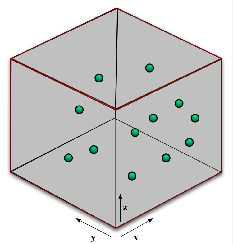
Fig. 28 A cubic volume of gas in thermal equlibrium#
Volume of gas in thermal equilibrium
Having looked at the Maxwell-Boltzmann distribution, and the theory of equipartition, we are now in a position to derive the pressure caused by a gas in thermal equilibrium. We are going to make one simplifying assumption; we are going to assume our gas consists of randomly moving, non-interacting particles. Such a gas is called an ideal gas. Because our ideal gas is in thermal equilibrium, the speeds of the particles follow the Maxwell-Boltzmann distribution and all the results we calculated for average energy etc. apply.
We’re going to think about a cubic box of gas, shown in figure 28. The force on the walls of our box is caused by the collisions of gas particles with the walls. During a collision the particles momentum is changed. The force felt by the wall is equal in size to the rate of change of momentum of the particles. Let’s look at just one wall of the box. Symmetry tells us the pressure must be the same on all walls of the box, so we can pick any wall we choose.
Let’s look at the right-hand wall. All of our gas particles are moving in three dimensions, but it is only the x-component of their velocity, \(v_x\), which causes them to hit this wall. When the particle hits the wall we assume the collision is elastic. This means that no kinetic energy is lost. Therefore, before the collision, the x-component of the particle’s velocity was \(v_x\); after the collision it is \(-v_x\). The change in momentum of the particle is
On average, the time taken between collisions with the right-hand wall will be the time it takes a particle with a x-velocity \(v_x\) to travel to the opposite wall, rebound and collide with the right-hand wall again. If our box has sides of length \(L\), this time is \(\Delta t = 2L/v_x\). The rate of change of momentum is thus
Since force is equal to the rate of change of momentum the force on the wall of the box is \(mv_x^2/L\). The pressure on the box wall is the force per unit area. The area of the box wall is \(L^2\) and so the pressure due to a single particle (labelled \(i\)), is
where \(V\) is the volume of the box. If we have N particles in the box, then we find the total pressure by adding up the contribution from all particles
Since \((v_{x,1}^2 + v_{x,2}^2 + \ldots + v_{x,N}^2) = N\bar{v_x^2}\), we can write
Our equation gives the pressure in terms of the x-component of the particle velocities. It would be more interesting to re-write it terms of the particle speed. We know that the speed, \(v\) obeys \(v^2 = v_x^2 + v_y^2 + v_z^2\). Also, since there is no preferred direction of motion for our particles the average velocities in the x, y, and z directions should all be equal, so \(\bar{v_x^2} = \bar{v_y^2} = \bar{v_z^2}\). Therefore we can write
Substituting this result into equation (19) we can replace \(v_x\) with \(v\) and obtain
The reason we have gone to all this trouble to write equation (20) in terms of the particle speed is that \(m\bar{v^2}\) is just twice the mean energy of the gas particles. But since the gas in in thermal equilibrium, the speed distribution is the Maxwell-Boltzmann distribution, and we worked out earlier that the mean energy of the gas particles was \(\frac{3}{2}kT\). So we substitute in \(m\bar{v^2} = 3kT\) to obtain
where \(n\) is the number of particles, per unit volume. This is the ideal gas law, which is hopefully familiar to you!
The ideal gas law is an equation of state for an ideal gas. An equation of state relates pressure, density and temperature. We made a starting assumption in our derivation; that the gas particles do not interact with each other. This is not true of real atoms and molecules, so we can expect the ideal gas law to be an approximation to the behaviour of real gasses. In fact, it is a good approximation up to very high densities and the ideal gas law is used widely in astrophysics. It is used, for example to describe the state of matter in the interiors of stars. Only when the gas density becomes extremely high can we no longer safely ignore the interactions between gas particles. For very compact objects (e.g white dwarfs and neutron stars) the ideal gas law breaks down and we need to derive new equations of state.
Radiation Pressure#
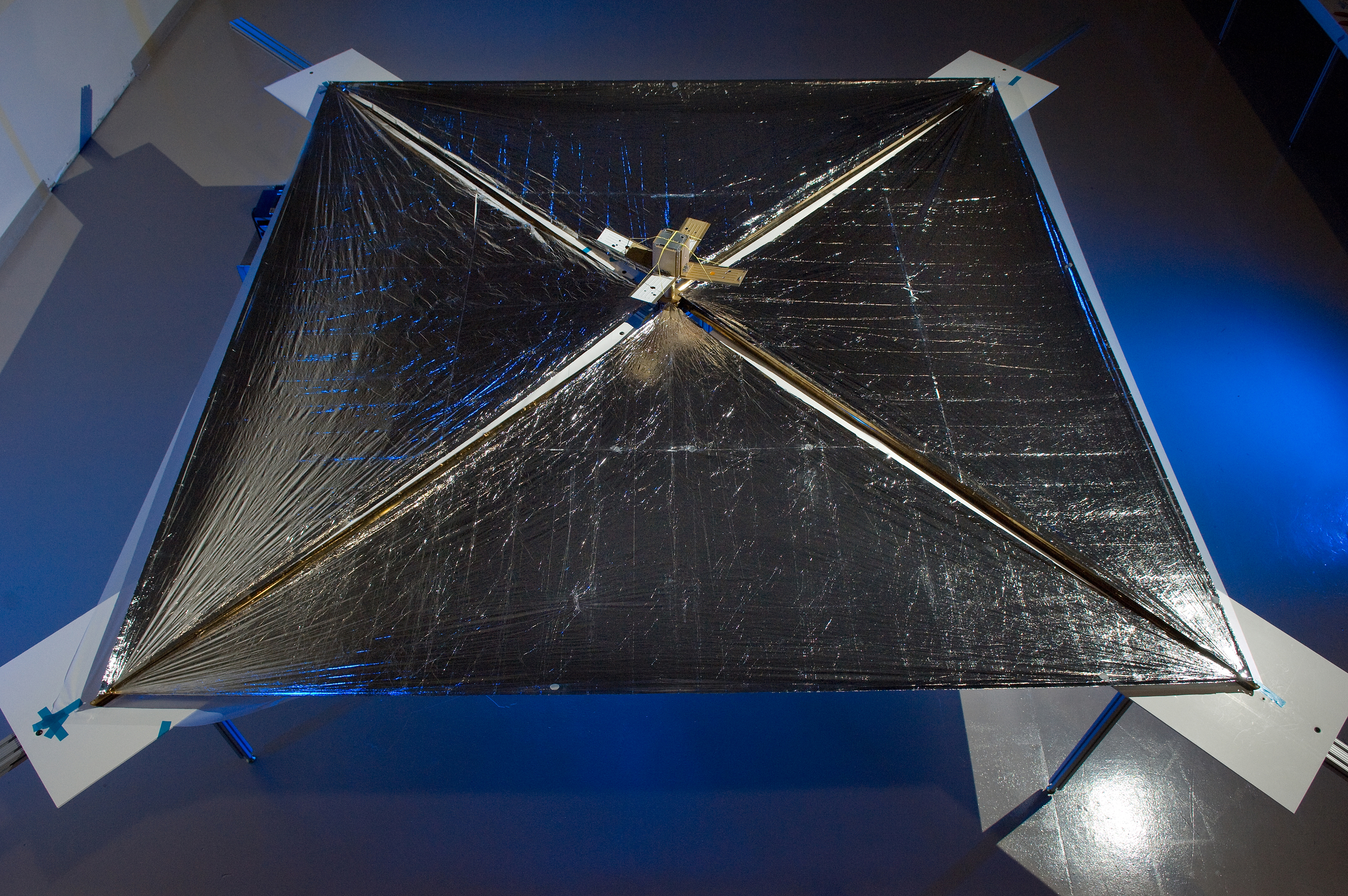
Fig. 29 NanoSail-D - a solar sail spacecraft designed by NASA to test methods of deploying solar sails for space travel. Unfortunately the spacecraft was lost in a launch failure of the rocket it was onboard.#
NASA’s NanoSail-D spacecraft
We saw in lecture 2 that photons also carry momentum. Remember, the momentum of a photon is \(p= E/c\), where \(E\) is the photon energy. Since photons carry momentum they too can exert a pressure. This pressure is, unsurprisingly, known as radiation pressure.
We could go through the derivation of the ideal gas law again, and replace our gas particles (with momentum \(mv\)) with photons (with momentum \(E/c\)). Rather than go through all the steps again, I shall just state the result
where \(a = 4\sigma/c\) (σ is Stefan-Boltzmann’s constant - \(5.67\times10^{-8}\) Wm-2K-1). Radiation pressure is generally a very small effect. Note however that it is strongly temperature dependent; radiation pressure is a significant effect in the highest mass stars, which are also the hottest stars. Radiation pressure is also the reason why solar sails (figure 29) could be used for long distance space travel. The radiation pressure on a solar sail is tiny, but over time it could accelerate a spacecraft to a reasonable speed. The great advantage is that no fuel need be carried, so the range of a solar sail spacecraft is unlimited!