
Spectroscopic Binaries#
What if we cannot resolve each of the stars individually? In that case, we cannot measure the orbit of the binary directly, but there is still a wealth of information that can be extracted from the spectra of binary stars. If the orbital motion has a component along the line of sight, a periodic radial velocity shift will be observable – remember, we can determine a stars radial velocity because the Doppler shift will change the wavelength of absorption or emission lines from the star – as shown in figure 62.
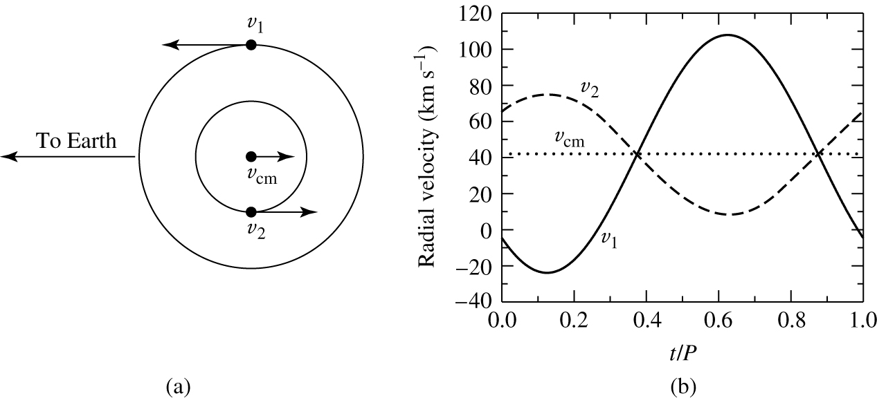
Fig. 62 The orbital paths and radial velocities of two stars in circular orbits. In this example, \(M_1 = 1\) M\(_{\odot}\), \(M_2 = 2\) M\(_{\odot}\) and the orbital period is \(P=30\) d. The whole binary is moving away from us with a radial velocity of \(v_{cm} = 42\) km s-1. \(v_1\) and \(v_2\) are the velocities of star 1 and star 2 respectively. (a) The plane of the circular orbits lies along the line of sight of the observer. (b) The observed radial velocity curves.#
Orbital paths and radial velocities of stars in a circular orbit
As with the visual binaries before, the angle of inclination between the line of sight and the orbit effects the observed radial velocities. Figure 63 shows that if the star has a velocity \(v\) around its orbit, what we actually observe is \(v^{\prime} = v \sin i\), where \(i\) is the inclination angle of the orbit. To obtain the actual velocities of the stars it is thus necessary to determine the orbital inclination somehow.
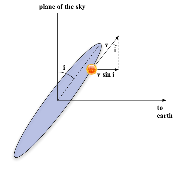
Fig. 63 A star follows a circular orbit in a binary with velocity \(v\). The orbit is inclined at an angle \(i\). This figure shows that the component of velocity along our line of sight - the radial velocity - is given by \(v \sin i\).#
Star in a circular orbit inclined to our line of sight
Double-lined binaries#
If both stars are comparably bright, we will be able to see absorption lines from both stars in the binary. Such a binary is called a double-lined spectroscopic binary (SB2). Double-lined binaries are very useful for mass determinations, as we will see below. We will assume the orbits are circular, in which case the speeds of the stars around the orbits are constant and given by \(v_1 = 2\pi a_1/P\) and \(v_2 = 2\pi a_2/P\). Since
we can use the formulae for the speed above to replace \(a_1\) and \(a_2\) with \(v_1\) and \(v_2\) to get
Hence, as for visual binaries we can determine the mass ratio without knowing the orbital inclination, in this case using the observed radial velocities, \(v_1^{\prime}\) and \(v_2^{\prime}\).
However, as is also the case with visual binaries finding the total mass of the binary does require knowledge of the orbital inclination. The total size of the orbit, \(a\), can be written as
We can use this to replace \(a\) in Kepler’s third law
and solve for the total mass,
Re-writing this in terms of the observed radial velocities, we find
Hence, provided we know some way of measuring the orbital inclination, double-lined spectroscopic binaries can yield individual stellar masses via radial velocity measurements.
Double-lined, eclipsing binaries#
Eclipsing binaries are the heavyweight champions of precise stellar measurements. In large part, this is because an eclipsing system tells us the orbit is very close to edge on. Put another way, if we see eclipses, we know the orbital inclination is close to 90°. Even if it were assumed that \(i=90^{\circ}\), while the actual value was close to \(i=75^{\circ}\), the resulting error in \(\sin^3 i\) would only be around 10%, with a corresponding error in the total mass. Thus, the observations of eclipses in a binary star’s lightcurve (figure 64) immediately allows us to roughly guess the orbital inclination, and get a decent estimate of the stellar masses.
We can get a better estimate of the inclination from the eclipse shape. Figure 64 shows the lightcurve of a binary with \(i=90^{\circ}\). When the smaller star is eclipsed by the larger one a nearly constant minimum occurs in the brightness of the binary as a whole. Similarly, even though the larger star is not completely eclipsed by the smaller one, a constant amount of area is obscured, and so again a nearly constant drop in brightness is observed. The eclipse is described as ’flat-bottomed’ and is a clear indicator of very high inclinations. When the inclination is a little lower, one star is not completely eclipsed by its companion. In this case, the minima of the lightcurve are no longer constant implying that \(i<90^{\circ}\).
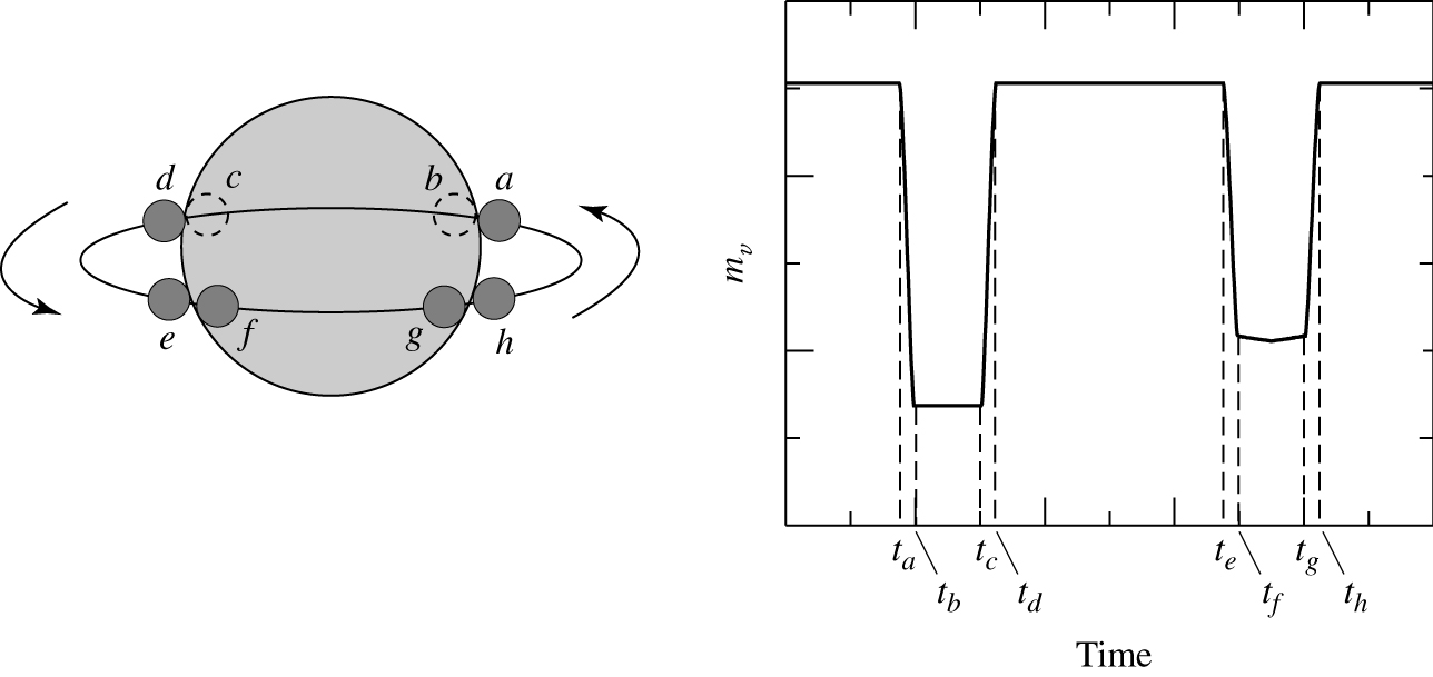
Fig. 64 Light curve of eclipsing binary at an inclination of 90 degrees#
Light curve of eclipsing binary at an inclination below 90 degrees
However, double-lined eclipsing binaries allow much more than just the stellar masses to be measured. Detailed analysis of the eclipse also allows direct measurements of the stellar radii, and the ratio of the effective temperatures to be measured. It is for these reasons that eclipsing binaries are so useful in stellar physics.
Stellar radii#
We refer again to figure 64 and looking at the binary with \(i=90^{\circ}\). Let us label the large star as star 1, and the smaller star as star 2. The relative velocities of the two stars is \(v=v_1+v_2\), so the time taken for the small star to move from \(a\) to \(b\) is \(t_b - t_a = 2r_2/v\). Since \(t_b-t_a\) can be measured from the lightcurve, we can immediately find the radius of the small star
Similarly, by considering the time take for the small star to move between \(b\) and \(c\), the size of the larger star can be determined
Effective temperatures#
By assuming the stars emit as black bodies we can find the ratio of the star’s effective temperatures. Recall that, for a black body the surface flux (energy emitted/second per unit surface area of the star) is given by \(F=\sigma T_{eff}^4\). The total light from the binary when both stars are visible is
When the small star (star 2) is full eclipsed the light from the binary is
When the larger star (star 1) is eclipsed most of the stellar disc is still visible, but an area equal to \(\pi r_2^2\) is obscured by the smaller star. The light from the binary is therefore
The depth of the eclipse when star 1 is eclipsed is \(L_T - L_1\). Likewise for star 2. A remarkable thing happens when we look at the relative depths of the two eclipses
which simplifies to
This is why double-lined eclipsing binaries are such a precious object for stellar astronomers. They are the only way to directly measure both the mass and radius of a star, and they also allow effective temperatures to be measured. Furthermore; notice that we did not need to know the distance to the star. All that is needed is observations of the radial velocity curves and the light curve. Unlike visual binaries, double-lined eclipsing binaries can yield measurements of the properties of stars which are too distant for a parallax measurement.
Single-lined binaries#
Obviously, the mass ratio and total mass can only be measured if the radial velocities of both stars are measurable. This requires that absorption or emission lines from both stars are visible in the spectrum of the binary. If one star is much brighter than the other the spectrum of the fainter star will be overwhelmed. Such a binary is called a single-lined binary (SB1). Recall that, for a double-lined binary,
and
Suppose that only star 1 is visible, so we can only measure \(v_1^{\prime}\). We can use the latter equation to replace \(v_2^{\prime}\) in the first equation with \(v_2^{\prime} = v_1^{\prime} m_1/m_2\) to give
Re-arranging terms gives
The right hand side of this equation is known as the mass function \(f(m)\). It only depends on observable quantities of a single-lined binary, the period and radial velocity of the visible component. The left-hand side of equation (47) is always less than \(m_2\), since \(m_1+m_2 > m_2\) and \(\sin i \le 1\). Therefore, the mass function provides a lower limit for the mass of the unseen component, \(m_2\). As we will see in the following case study - this can still be very useful.
Single-lined binary case study: black holes#
Black holes are objects whose gravity is so intense that nothing can escape, not even light. One way of looking at this is a black hole’s escape velocity is greater than the speed of light. The escape velocity is given by equation (42);
Therefore, by setting the escape velocity equal to \(c\), we can find an equation for the Schwarzchild radius,
Anything within the Schwarzchild radius of a black hole cannot escape; we can think of the Schwarzchild radius as the ’size’ of the black hole itself.
But how do we know black holes exist. If no light can escape them, and all our knowledge in astronomy comes from measuring light, how can we be sure they are not just figments of our imagination?
Up until recently, evidence for black holes has come from a type of single-lined binaries called X-ray binaries. X-ray binaries are binary stars in which a solar-type star orbits a compact object (either a neutron star or a black hole). The orbits of these binaries are so close together that the compact object rips gas off the surface of the solar-type star and the gas falls onto the compact object. So much energy is released in this process that the gas heats up to several hundred million degrees and so radiates in X-rays: Remember Wien’s Law - \(\lambda_{max} = 2.898\times10^{-3}/T\).
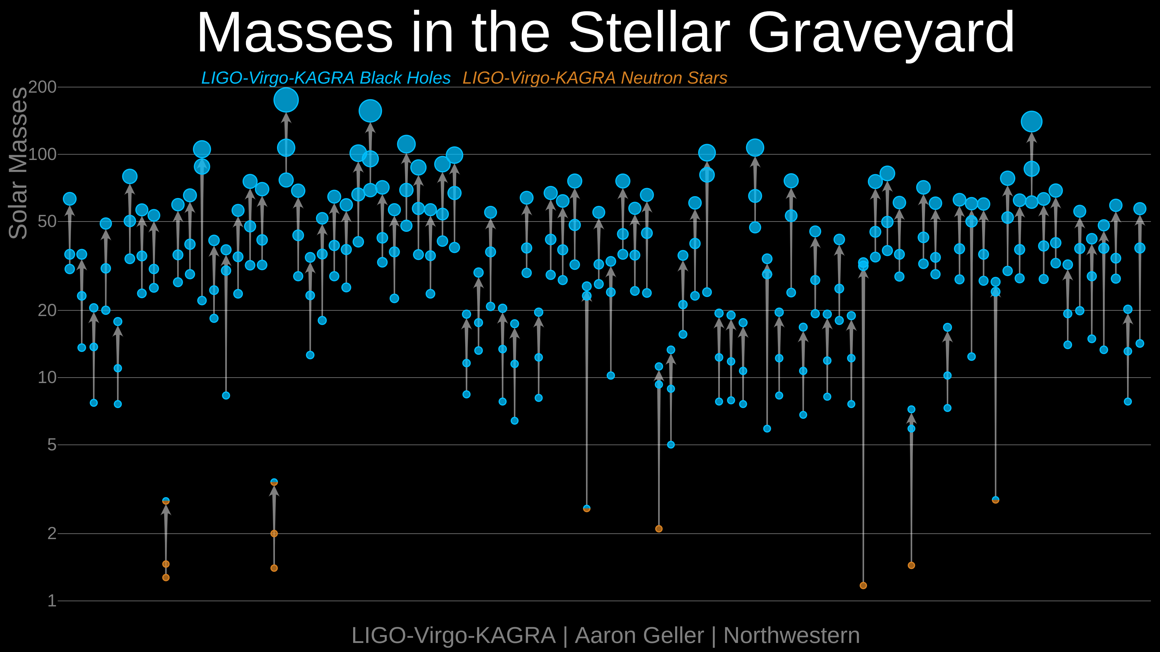
Fig. 65 LIGO-Virgo-KAGRA have discovered a new population of black hole (blue) and neutron star (orange) mergers. Credits: LIGO/VIrgo/KAGRA/Northwestern Univ./Aaron Geller#
LIGO-Virgo black hole and neutron star mergers
The spectrum of the neutron star or black hole in an X-ray binary is never visible, because the compact object is small and faint compared to the companion star. X-ray binaries are single-lined spectroscopic binaries. However, we can measure the mass function and obtain a lower limit for the mass of the compact object. Since neutron stars have a maximum mass of \(2.5-3\,M_{\odot}\), if the compact object weighs more than this it must be a black hole! The first black hole inferred from this method was Cyg X-1 based on spectroscopic monitoring by Louise Webster and Paul Murdin in 1972. Over a dozen X-ray binaries are now known with mass functions greater than 3\(M_{\odot}\). Since the mass function is a lower limit to the mass of the compact object, these binary systems must contain black holes.
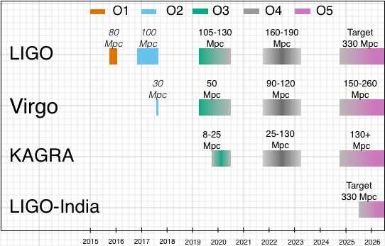
Fig. 66 Schedule for the first five gravitational wave observing runs for LIGO, Virgo, KAGRA and LIGO-India, through to 2026, as of July 2019.#
Observing schedule for LIGO, Virgo, KAGRA and LIGO-India through to 2026
This indirect evidence for black holes has recently been supported by the discovery of merging stellar mass black holes through gravitational waves with LIGO and Virgo observatories. The first detection was achieved by LIGO in September 2014 (GW150914), involving the merger of 36 and 29 solar mass black holes, which led to the 2017 Nobel prize for physics being awarded to Rainer Weiss, Barry Barish and Kip Thorne. Merging neutron stars were first identified in August 2017 (GW170817), the nature of whose remnant remains uncertain. The census of LIGO-Virgo compact mergers as of Dec 2021 is shown in Fig. 65, in which gravitational wave sources were being identified at a rate of 1/week in LIGO/Virgo/KAGRA observing run 3 which ran from 2019–2020 (see Fig. 66)), and are reported through an app.
In April 2019, the Event Horizon Telescope, a consortium of world-wide radio telescopes exploiting a technique known as very-long-baseline interferometry (VLBI) reported the first image of a supermassive black hole in the centre of M87, which is the central galaxy in the Virgo cluster, shown in Fig. 67. The mass of this supermassive black hole is thought to be 6.5 billion solar masses. EHT radio observations of Sgr A*, the supermassive black hole at the centre of our own Galaxy followed in May 2022.
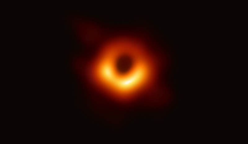
Fig. 67 Event Horizon Telescope observations of the supermassive black hole in the centre of M87, a massive elliptical galaxy in the Virgo cluster. Credit: Event Horizon Telescope Collaboration.#
EHT observations of the supermassive black hole in M87
Exoplanets#
The planets of our solar systems have been recognised since the Babylonians, since nearly 2000 years BC. In the four millenia that followed they were the only planets known to exist. Then, on October 6\(^{\rm{th}}\) 1995, Michel Mayor and Didier Queloz announced the discovery of a exoplanet orbiting the main-sequence star 51 Peg. This discovery started a new era of planet discovery; as of Feb 2025 there are 7,412 known planets outside our solar system - for current values see Catalogue of Exoplanets.
Exoplanets were first discovered and characterised by measuring the radial velocity of the star as it orbits the centre of mass of the star-planet system. This radial velocity of the host star is often called a Doppler wobble. To date, the vast majority of exoplanets have been discovered by looking for stars which show a detectable Doppler wobble. Another way of searching for exoplanets is to look for the tiny dip in light caused by the planet passing in front of the host star - an exoplanetary transit. Transit searches have become a popular alternative to the Doppler wobble technique for exoplanet hunting. Transit searches have a number of advantages. Because many stars can fit on a CCD image, many more stars can be studied in a given time. Also, because the starlight is not being divided into many wavelengths for study, quite small telescopes can be used - in contrast to the Doppler wobble technique which uses the biggest telescopes available.
Exoplanets as single-lined binaries#
The planets themselves are extremely difficult to see directly; exoplanetary systems are therefore a type of single-lined spectroscopic binary, and can be analysed and treated as such. We measure the Doppler wobble of the planetary host, and can construct the mass function, as given by equation (47),
where the subscript \(p\) denotes the exoplanet and the subscript \(s\) denotes the host star. However, the mass of the star is much greater than that of the planet (Jupiter, for example, is around 1000 times less massive than the Sun); we can use this to re-write the mass function in a much more useful form. The term \(m_p + m_s\) can be written as
because \(m_p/m_s \ll 1\). Substituting \(m_p + m_s \approx m_s\) into the mass function, we get
It is normally possible to get a good estimate of the stellar mass, \(m_s\). This is because, on the main-sequence, there are well known relationships between a star’s mass and a number of observable quantities, such as its luminosity, effective temperature, or spectral type. So by measuring (for example), the spectral type of the host star, we can estimate the stellar mass to an accuracy of a few percent. Armed with an estimate of the stellar mass and Doppler wobble measurements of the host star (which reveal both the observed radial velocity \(v_s^{\prime}\) and the period \(P\)), we can calculate the quantity \(m_p \sin i\), which is a lower limit to the mass of the planet.
Doppler wobble measurement#
The majority of the known exoplanets have been found by searching for Doppler wobbles in nearby stars, and as outlined above, the Doppler wobble gives a lower limit to the planetary mass. But how large is it? Consider the Doppler wobble of the Sun, as caused by Jupiter. The period of Jupiter is 11.86 years, and it’s mass is 1.9\(\times 10^{27}\) kg, compared to the Sun’s \(2\times10^{30}\) kg. Putting these quantities into equation (48), and assuming that \(i=90^{\circ}\), so all of the stellar motion is along our line of sight, we find a Doppler wobble of around 12 ms-1. To put this in some sort of context, that’s just less than 30 mph. To detect exoplanets thus needs us to be able to measure radial velocities of objects which are many parsecs away, and moving away from us at a similar speed to city centre traffic!
Such observations are extremely challenging, and this explains why the discovery of exoplanets was so recent. The problem lies in calibrating a spectrograph. If you measure the spectrum of a planet-hosting star you need to measure the wavelength of the absorption lines to measure the Doppler shift. What you actually measure is the position of an absorption line on your detector, and there are lots of flaws in the instrument that can cause this to change, even if the star itself shows no motion. For example, the spectrograph can flex as the telescope moves, or as the instrument cools during the night. To get round this, astronomers calibrate their spectrographs, by observing lamps which emit lines of known wavelength. In conventional spectrographs this is done every hour or so. The calibration usually limits accuracies to a few km/s: much worse than we need to detect exoplanets! To get round this, spectrographs have been built where the starlight shines through an Iodine cell before the spectrum is measured. The Iodine superimposes absorption lines on the star’s spectrum. The position of the star’s absorption lines can then be measured relative to the Iodine lines. This greatly improves precision, and the best spectrographs can reach radial velocity accuracies of 1 m/s; a slow walking pace!
Planets found from Doppler Wobble: observational bias#
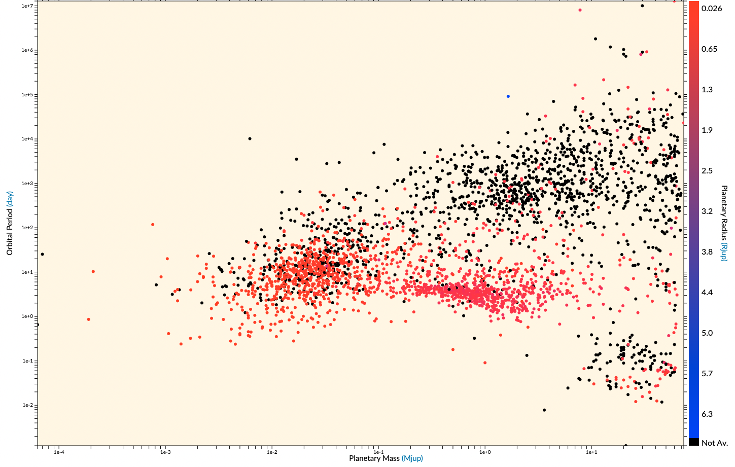
Fig. 68 Properties of 7412 known exoplanets as of 4 Feb 2025, colour coded by planetary radius. The y-axis shows orbital period while the x-axis shows the planetary mass (we assume mass is equal to the minimum mass given by the mass function).#
Properties of known exoplanets
Figure 68 shows the properties of all 7412 exoplanets detected as of 4 Feb 2025. The known exoplanets are totally unlike the planets in our own solar system. Most of the known exoplanets are of a similar mass to Jupiter, and yet have orbits similar to that of Earth. Some exoplanets (so-called hot Jupiters) are similar in mass to Jupiter, but have orbits smaller than Mercury’s! This raises the immediate question of whether these planets are typical or not.
There is good reason to suspect they are not, because planet-hunting using Doppler wobble is very strongly biased. Look in detail at equation (48). In order for the Doppler wobble \(v_s^{\prime}\) to be large we need the mass of the planet \(m_p\) to be large, and the period \(P\) to be small! A small period implies a small orbit – Kepler’s third law says that \(P^2 \propto a^3\) – so it is hardly surprising that the Doppler wobble technique is finding lots of heavy planets orbiting close to their host stars. Note also that there are almost no planets found using the Doppler wobble technique with orbital periods longer than 10 years. This is because we need to see the radial velocity curve repeat itself in order to measure the period and be sure we are seeing an exoplanet orbiting the star. Since we have been monitoring stars for only 15 years or so, it is natural that exoplanets with long periods are rare! Exoplanet searches are steadily becoming more accurate and as time goes on it is hoped we will start to find exoplanetary systems more like our own Solar system.
Transiting exoplanets#
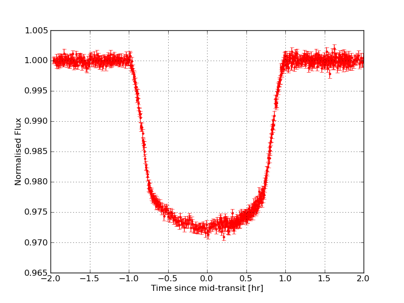
Fig. 69 Transit of exoplanet Wasp-4b in front of its host star.#
Transit of exoplanet Wasp-4b
Recall the mass function for planetary systems,
Obviously, to get more than a minimum mass for the exoplanet we need to know the orbital inclination. By comparison to spectroscopic binaries, the obvious way to do this is to look for systems in which the exoplanet passes in front of the host star. In stellar binaries these are called eclipses; in exoplanet systems, they are known as transits (e.g. Wasp-4b transit in Figure 69).
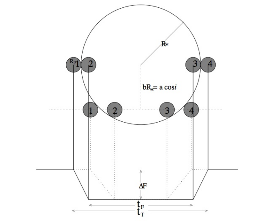
Fig. 70 How the inclination affects the transit shape. The solid line shows the transit shape for i=90°, whilst the top shaded circles show the position of the planet at beginning and end of the ingress and egress from transit. The dashed line shows the transit shape for a lower inclination, and the lower row of circles shows the planetary positions at ingress and egress. Transits at lower inclinations last for shorter times, and have slower transitions into and out of transit.#
Impact of inclination on transit shape
As with spectroscopic binaries, the presence of transits allows us to measure the inclination, and more besides. Again, in a similar way to eclipsing binaries, the presence of transits tells us that the inclination is close to 90°, and this might be enough for our needs. If not, the detailed transit shape tells us the precise inclination, as shown in figure 70. The transit depth can also tell us the radius of the exoplanet. The luminosity of the star/exoplanet system outside of transit is just given by the luminosity of the star. Assuming the star radiates as a black body this is given by
During transit, the exoplanet blocks some of the surface of the star. The visible surface area of the star is now \(\pi (r_s^2 - r_p^2)\), so the luminosity during transit is
Now, we calculate the transit depth, as a fraction of the total out-of-transit light
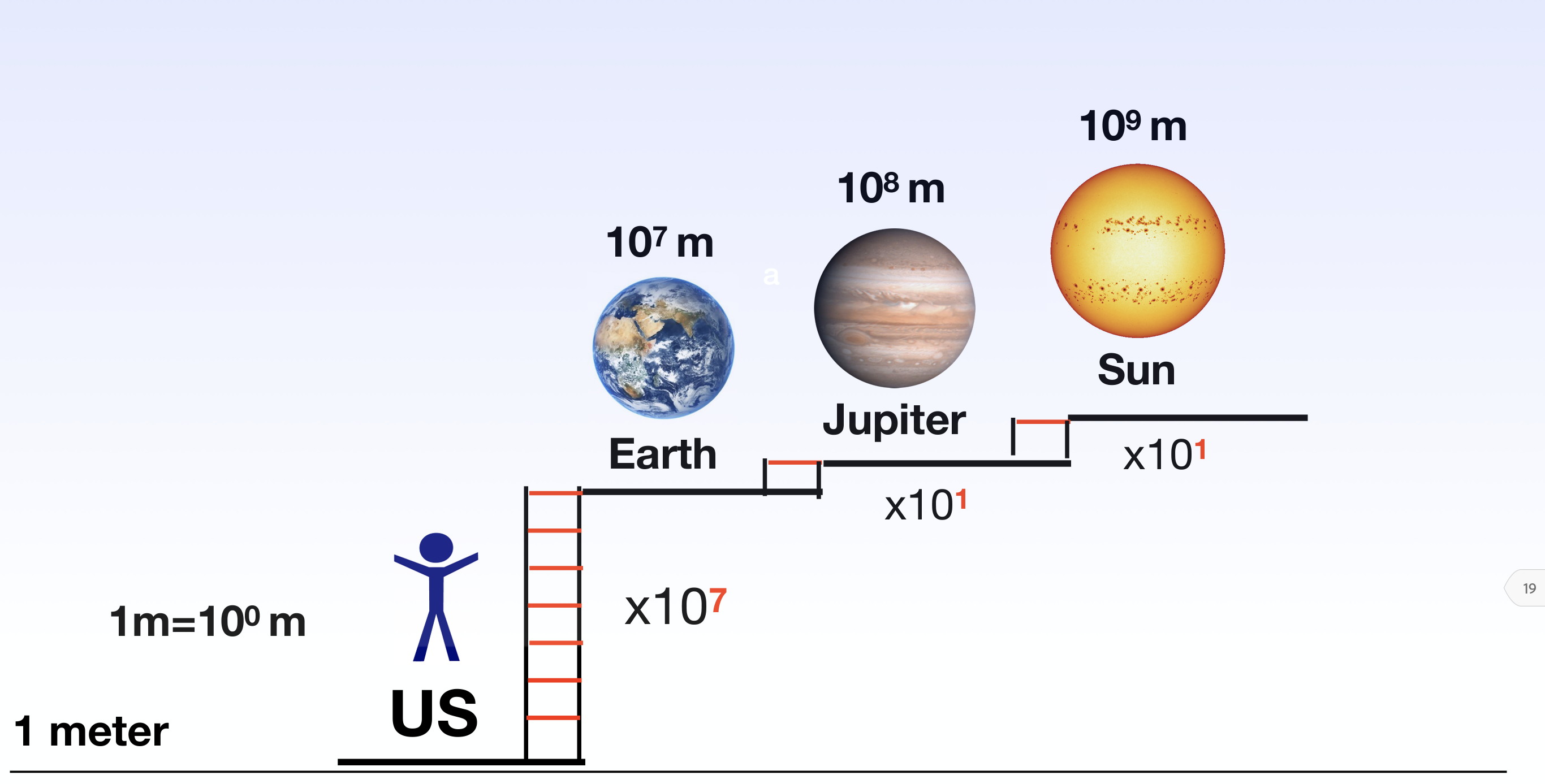
Fig. 71 Reminder of the size of terrestrial planets such as the Earth, versus gas giants (Jupiter) and main sequence stars, such as the Sun. Courtesy Stan Owocki (Bartol).#
Size of Earth, Jupiter, Sun
Using equation (49) we can measure the planetary radius using the transit lightcurve. We need to know the radius of the host star but this, like the mass of the host star earlier, can be estimated from the spectral type and main-sequence mass-radius relationships.
Note that equation (49) predicts that transit depths are very small - normally only 1 or 2% of the total light from the star. Measuring planetary transits thus requires very accurate photometry, and transit searches are inevitably biassed towards larger planets, which cause the biggest transits. The transit depth does not depend on the distance of the planet from the star; unlike the Doppler wobble searches, transit searches are sensitive to planets in large orbits around their host stars. They are still slightly biased against these planets though; planets in large orbits are less likely to show transits in the first place. The dependence of transit depth on the planetary radius means that detecting Earth-like planets needs better accuracy than can be obtained from the ground - see Fig. 71. To get round this, several satellites aimed at transit searches have been launched. Examples include Kepler, TESS and CHEOPS satellites. These offer a good chance of detecting a truly Earth-like planet within the next few years. Nevertheless, Kepler has revealed a deficit in short period planets between super-Earths (up to 1.5 Earth radii) and sub-Neptunes (above 2 Earth radii), known as the radius valley.
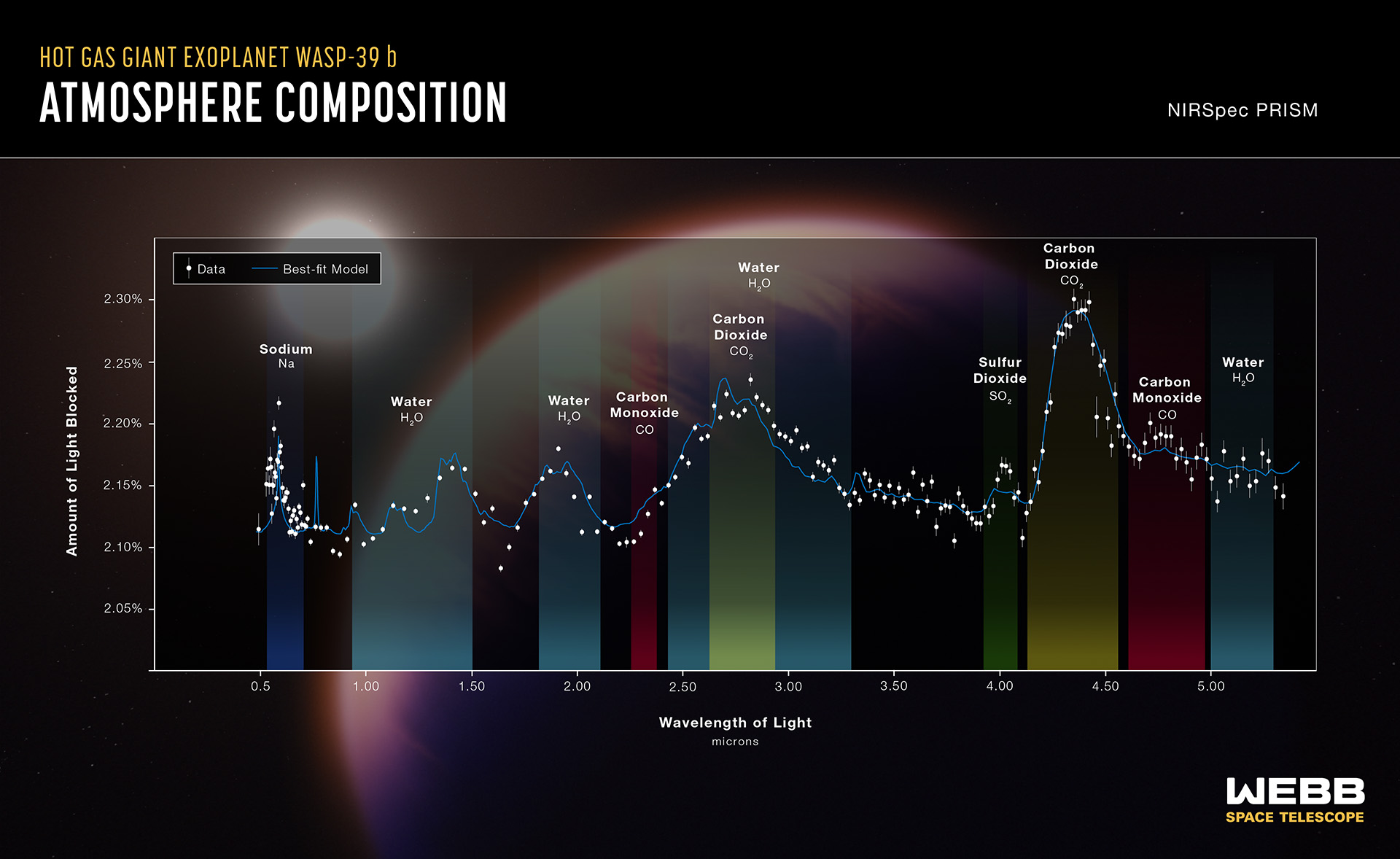
Fig. 72 JWST near infrared transmission spectroscopy of the exoplanet WASP 39b showing an atmospheric composition including water and carbon monoxide/dioxide. Credit: NASA, ESA, CSA, Joseph Olmsted (STScI).#
Transmission spectroscopy of WASP 39b
In the meantime, transmission spectroscopy of exoplanets has been undertaken with Hubble and most recently JWST, permitting a determination of atmospheric abundances in exoplanetary atmospheres from comparisons between spectroscopy obtained during transit and unfiltered starlight. An example of JWST transmission spectroscopy of exoplanet WASP 39b is presented in Fig. 72, showing an atmospheric composition including water, CO and CO2. It is also possible to obtain direct spectroscopy of planetary mass companions at large angular separations from their hosts, as shown in Fig. 73 for a \(\sim 20 M_{\rm Jup}\) companion to an M-dwarf binary system at 22 pc (\(\sim\)150 AU separation).
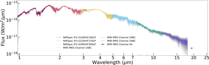
Fig. 73 JWST infrared spectroscopy of the planetary mass companion (VHS1256b) to an M-dwarf binary (d= 22 pc), at a separation of 8 arcsec (150 AU). Miles et al. 2023 (ApJL 946 L6).#
JWST spectroscopy of planetary mass companion VHS1256b
Weighing Galaxies#
So far we have measured the mass of planets in our own Solar system, planets around other stars and stars in various types of binary systems. Now we take a step up in scale, and ask how we can measure the mass of galaxies.
Galaxies have been known since the 10th century, but their nature was only recently understood. The idea that galaxies were disks of stars, like our Milky Way has been around since the mid-18th century. However, it was also thought possible that nebulae, as galaxies were then called were bright clouds of gas and dust within the Milky Way itself. As we discussed earlier, the matter was finally resolved in the 1920’s, when astronomers used Cepheid variables to measure the distances to nearby galaxies.
Of course, galaxy masses are measured using the effects of gravity, but unlike stars and planets, we can measure the mass of a single galaxy, even if it is isolated in space. This is because we can use the rotation of the galaxy, to measure the mass.
Galaxy rotation#
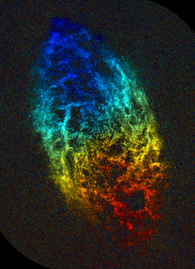
Fig. 74 21cm radio image of M33 (Triangulum) from the Very Large Array and Westerbork Synthesis Radio Telescope, illustrating the galaxy’s rotation#
21cm radio observations of M33 illustrating the galaxy’s rotation
Spiral galaxies, like the Milky Way, rotate. Due to the Doppler shift, light from one side of the galaxy will appear blueshifted, whilst light from the other side of the galaxy appears redshifted (see figure 74 from NRAO). By measuring how the rotation speed changes with distance from the galaxy centre, we can measure the mass of the galaxy. Before we show how that works, we should quickly discuss how the rotational velocity is measured.
The visible light from galaxies is dominated by stars. Therefore, the optical spectrum of a galaxy looks like the spectra of lots of stars added together, and contains many absorption lines that can be used to measure the Doppler shift. However, there is more to the galaxy than just starlight; galaxies also contain significant amounts of gas and dust; which can extend well beyond the regions of the galaxy that contains stars. Since hydrogen is the most abundant constituent of this gas, we can track the motion of this gas using hydrogen lines, but not the hydrogen lines which appear in the optical and ultraviolet (the Balmer, Lyman and Paschen series). Remember that absorption and emission lines are created when electrons hop between allowed energy levels in an atom. These energy levels are labelled with a principal quantum number, \(n\). In earlier lectures we stated that all energy levels with the same value as \(n\) had the same energy. This is not quite true. It turns out there is a tiny, tiny difference in energy between electron orbits in which the electron and proton spin in the same direction, and orbits in which the electron and proton spin in opposite directions. This phenomenon is known as hyperfine splitting. The difference in energy is \(9.5\times10^{-25}\) J, and electrons changing from one level to another give rise to light with a wavelength of 21 cm. This is in the radio region of the electromagnetic spectrum. Thus, optical spectroscopy tells us about the rotation speeds of those parts of the galaxy which contain stars, and radio spectroscopy tells us about the rotation of the parts of the galaxy where stars are absent.
Galaxy rotation curves#
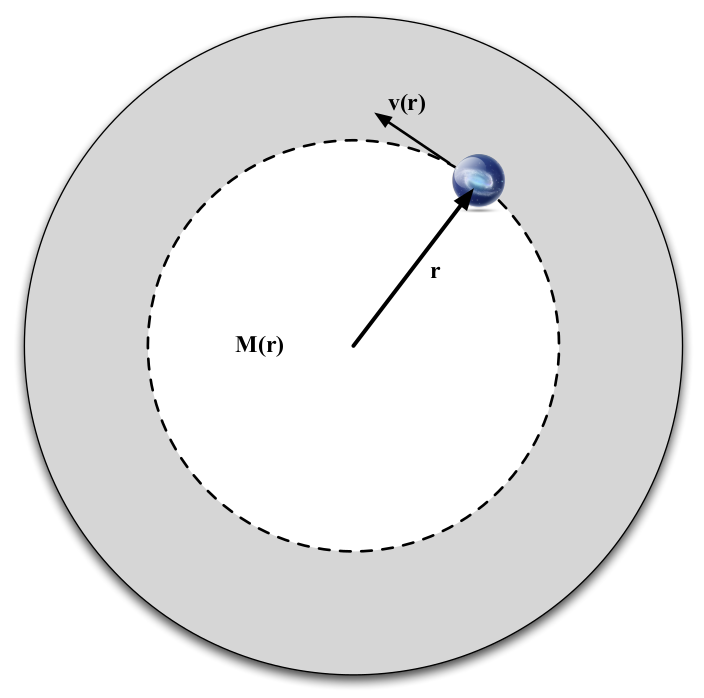
Fig. 75 A simple model of galaxy rotation#
Simple model of galaxy rotation
Before we look at the observed rotation of galaxies, let us work out what we expect to see. We look at the rotation under gravity of material a distance \(r\) from the centre of the gravity. We assume that the mass inside \(r\) and outside \(r\) is distributed spherically. Our simple model is shown in figure 75. To calculate the expected rotation, we need to remember two theorems we proved at the end of Chapter 10. One was that the gravity due to the mass inside \(r\) is the same as if all that mass was concentrated in a point at the centre of the galaxy. The other was that the mass outside \(r\) exerts no net gravitational force. We can find the rotation of material at \(r\) by balancing the force from gravity and the acceleration of the material (assuming it is on a circular orbit). This gives
. where \(M(r)\) is the mass inside \(r\), \(m\) is the mass of a small test mass at \(r\), and \(v(r)\) is the rotational speed at \(r\). Re-arranging gives
Let’s assume the galaxy has a constant density. Inside the galaxy
Substituting this back into equation (50) tells us that the rotational velocity should increase linearly with radius, \(v(r) \propto r\). Outside the galaxy, the \(M(r)\) is constant (no more mass is enclosed by spheres of larger radii). This suggests that outside the galaxy, the rotation speed should slowly drop off as \(v(r) \propto r^{-1/2}\).
A graph of rotation speed \(v(r)\) versus radius \(r\) is known as a galaxy rotation curve, and our calculations predict it should look like the red line in figure 76.
Actual galaxy rotation curves#
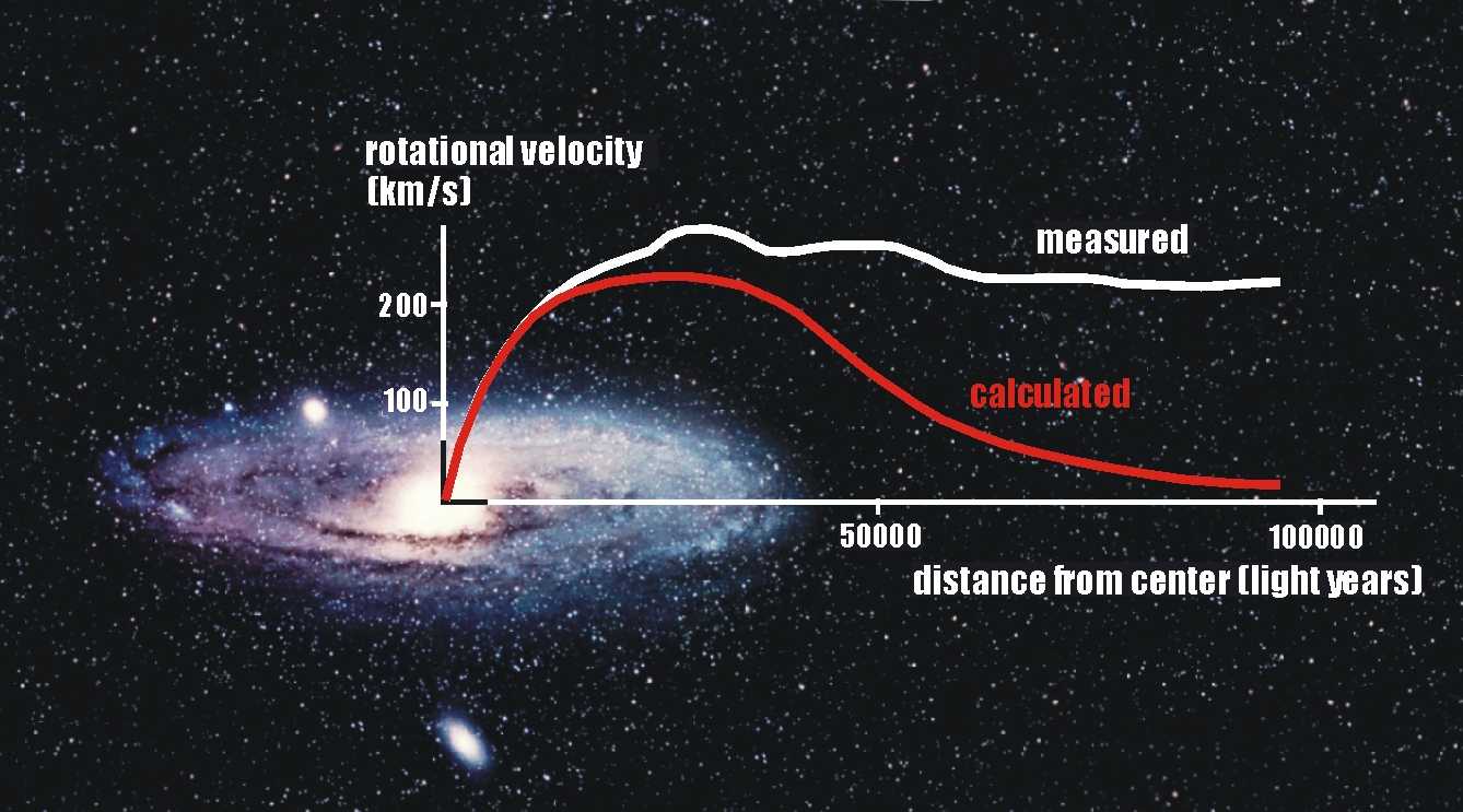
Fig. 76 A sketch of actual versus predicted rotation curves for a spiral galaxy#
Sketch of predicted versus measured galaxy rotation curves
The first indication that real life doesn’t follow our simple calculation came from the Swiss astronomer, Fritz Zwicky, in the 1930’s. Zwicky is an amazing character; an outspoken man who considered “humbleness a lie”, he was not liked by his colleagues. Indeed, he referred to his colleagues as “spherical bastards”, because they were “bastards, whichever way you looked at them”. Perhaps because of his unpopularity, Zwicky is often not credited for discoveries to which he can rightly claim priority. A prime example is that, in the 1930’s, Zwicky showed that the motion of galaxies seemed to be at odds with what one would expect from theory.
Figure 76 shows the predicted, and actual, rotation curve of a spiral galaxy. As seen above, theory predicts that the rotation speed should drop with increasing radius. Instead, the rotation speed is roughly constant, even out to distances well beyond the radius which contains all the visible starlight. From equation (50) it is obvious that a flat rotation curve implies that \(M(r) \propto r\). Since \(M(r)\) increases with \(r\), even at these large radii, there must still be material there. In other words, even at radii well outside the visible extent of the galaxy, there is still large amounts of matter.
Unsurprisingly, Zwicky labelled this material “Dark Matter”, since it was not visible, except through its gravitational influence. This was a major discovery which might have revolutionised astronomy at the time. Naturally, Zwicky’s colleagues ignored it, until the effect was once again discovered forty years later, pioneered by Vera Rubin
How much of galaxies is dark matter? When we measure the rotation of galaxies, we actually observe \(v^{\prime}(r) = v(r) \sin i\). If we know the inclination of the galaxy, we can work out the true mass of the galaxy. We can estimate the total amount of mass contained within the visible components of the galaxy (e.g stars) by measuring the luminosity, and working out what mass of stars is necessary to create that luminosity. This only accounts for 10-20% of the total mass of the galaxy, as measured from the rotation curves. Therefore, something like 80-90% of the mass of galaxies is contained in dark matter.
Giant galaxies, such as the Milky Way, have masses of 10\(^{12-13} M_{\odot}\), intermediate mass galaxies, such as the Large Magellanic Cloud or M33 have masses of 10\(^{10-11} M_{\odot}\) while typical dwarf galaxies such as the Small Magellanic Cloud have masses of 10\(^{8-9} M_{\odot}\). Some ultra-faint satellite galaxies of the Milky Way have masses as low as 10\(^{6-7} M_{\odot}\) which overlap with massive star clusters (e.g. ω Centauri Globular Cluster) although they are an order of magnitude larger and are dominated by dark matter rather than baryonic matter (stars).
Dark Matter#
What is dark matter? We know that is has mass, and that it does not emit light. This does not rule out the possibility that dark matter is made out of the same stuff as ordinary matter. Black holes, for example, have mass and emit no light by definition. Very low mass stars and brown dwarfs do emit some light, but they are so faint as to be invisible at the distances of nearby galaxies. Perhaps dark matter is made of large numbers of brown dwarfs, in the outer regions of galaxies? We can test this prediction by carrying out extremely deep searches for brown dwarfs in the outer regions of our own galaxy. Such studies reveal that brown dwarfs only constitute around 6% of the dark matter in our own galaxy. Black holes can be searched for by gravitational lensing. Einstein predicted that gravity bends light. If a black hole passes between us and a background star, its gravity will bend the light from the background star in a distinctive way. Studies using gravitation lensing have shown that black holes are not a big component of dark matter.
We are left with the possibility that dark matter is made of material entirely unlike normal matter. Dark matter particles must be made of particles which create and feel gravity, but interact only very weakly with light and normal matter. These particles are called WIMPs - “weakly interacting massive particles”. As yet, no-one has actually managed to detect a WIMP directly, so we know very little about their properties. Nevertheless, the search is currently ongoing, so next year the story may be different.
Galaxy Clusters#
Galaxies are often not alone in space. Instead they tend to form large clusters of galaxies. How much do these clusters weigh? A while back, we discussed the thermal properties of matter, and derived the equipartition theorem, which states that matter in thermal equilibrium has \(1/2 kT\) of thermal energy for every degree of freedom. I also said that this could be used to solve difficult problems in astrophysics. The equipartition theorem is a closely related to another theorem for systems in equilibrium, known as the virial theorem. The virial theorem states that the kinetic energy of a large, self-gravitating system is minus \(1/2\) its gravitational potential energy, or
A cluster of galaxies is a large, self-gravitating system, and we can apply the virial theorem to measure the mass of the cluster.
We assume for simplicity that the cluster is a sphere of radius \(R_c\), containing \(N\) galaxies, all with the same mass \(m\). The kinetic energy of galaxy \(i\) is \(m v^2_i/2\), so the total kinetic energy of the cluster is
where \(M_c = Nm\) is the total mass of the cluster. Previously, we derived equation (41) for the gravitational potential energy of two masses,
For a spherical collection of galaxies, the gravitational potential energy is hard to work out, but is approximately given by
Applying the virial theorem, we find that
Of course, we cannot measure the true speeds of the galaxies. Instead, we use the Doppler shift to measure the radial velocity of each galaxy \(v_r\). On average, a galaxy is as likely to be moving along our line of sight, as in the other two directions (\(\theta, \phi\)), and so \(<v^2_r> = <v^2_{\theta}> = <v^2_{\phi}>\). Hence we can write \(3 <v^2_r> = <v_2>\), which gives
Re-arranging for the mass of the galaxy cluster gives
Masses measured in this way are known as virial masses. An appropriate value for the size of the cluster must be adopted. This comes from combining the angular size of the cluster with a distance estimate (from Hubble’s law and the redshift of the cluster). When we calculate the virial masses of clusters, we find once again that most of the mass of the galaxy cluster is not explained by the amount of visible material. As well as being a major component of the galaxies themselves, it seems the space between galaxies is also full of dark matter!
On a still larger scale, Fig. 77 shows results of the EAGLE cosmological simulation in which hot gas is contained within dark matter structures that seed galaxies.
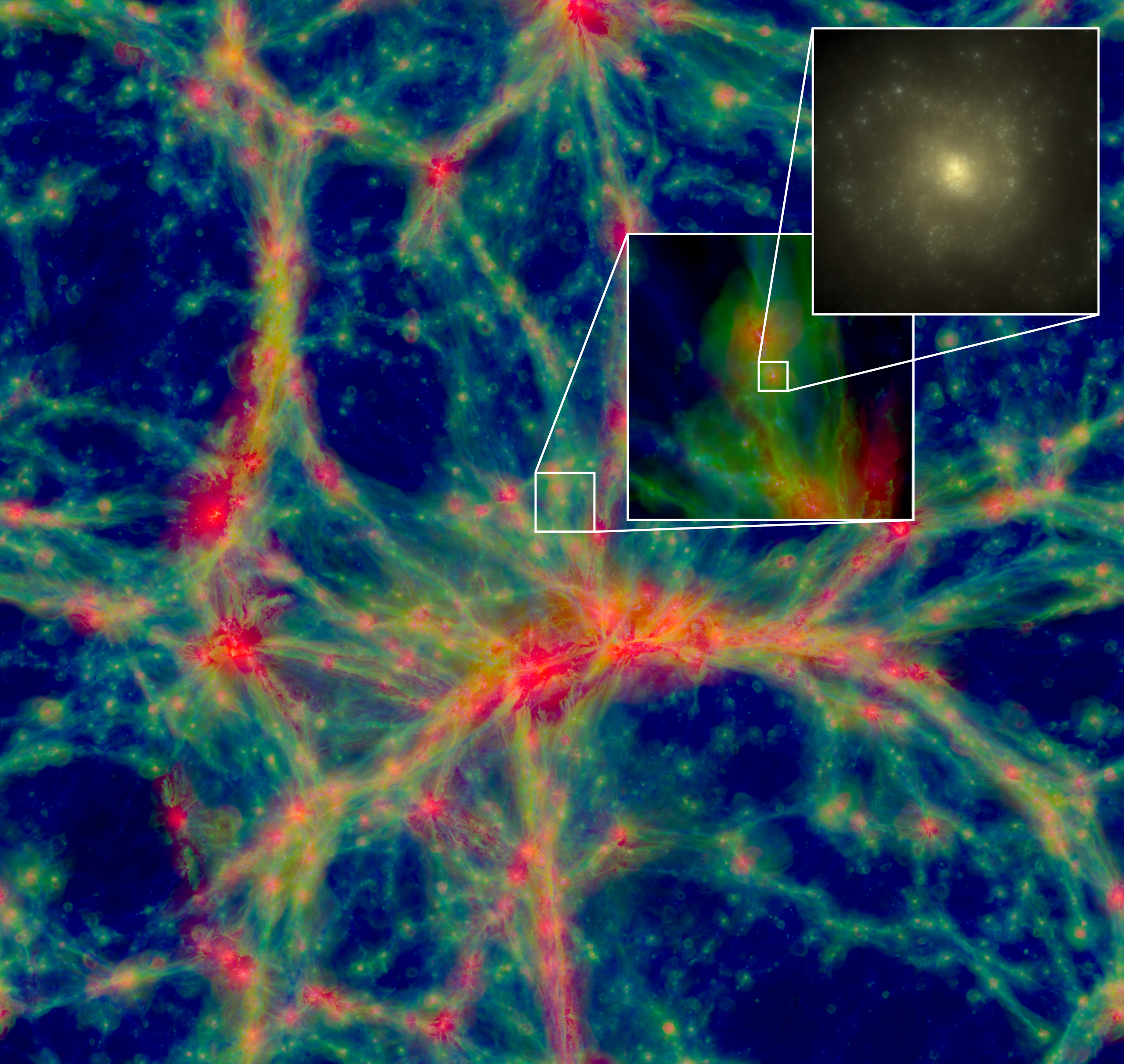
Fig. 77 EAGLE cosmological simulation illustrating the dark matter structures thought to permeate the universe, together with inset.showing a Milky Way-like galaxy in gas and stars#
Cosmological simulation of Dark Matter structures