Chapter 10: Gravitational astrophysics

Throughout this course, I hope you have been struck by how astronomy is a science of remote sensing; using our understanding of physics we can interpret the observations we make of the night sky, and deduce from them facts about the objects of our study. In no area of astrophysics is this more apparent than when we use Newton’s law of gravity to understand the motions of objects in gravitationally bound systems (for example, binary stars, galaxies, planetary systems). The application of gravity leads to some of the most subtle and elegant measurement techniques in astrophysics. We will spend the remainder of the course studying these techniques, so we had better have a firm grasp of gravity itself.

History

The accepted view of our place in the Universe in the 16th Century remained the ancient geocentric model of Ptolomy, despite the heliocentric theory advocate by Copernicus. Towards the end of the century, the Danish nobleman Tycho Brahe was busy accumulating a huge collection of observations of the Solar System. As the official astronomer to the Holy Roman empire, Brahe had the best observatory in the world, and was credited with taking the most accurate astronomical observations of the time (telescopes had not yet been invented). As well as being famous for the painstaking accuracy of his work, Brahe is also famous for his nose. Having lost part of his nose in a duel, Brahe replaced it with a prosthetic nose made of copper. Tycho favoured a mixed geo-heliocentric model for the Solar System.

Brahe’s observations were put to good use by Johannes Kepler; a German mathematician and astronomer who was, for a time, Brahe’s assistant. Kepler wanted to deduce the rules which governed the Solar System; rules which he believed were created by God. He used Brahe’s observations to tease out 3 laws which all bodies in the Solar System obey, supporting the heliocentric model. Kepler’s laws were not a physical theory; there was no framework in place to understand them. Instead they were a tour-de-force of empirical deduction. Around the same time, Galileo Galilei developed telescopes which permitted the discovery of Jupiter’s largest moons, so also favoured the heliocentric model. Kepler’s laws are still used by astronomers today, and played a crucial role in the development of a theory of gravity.

Kepler’s Laws

The 1st Law

“The orbit of every planet is an ellipse with the Sun at a focus”

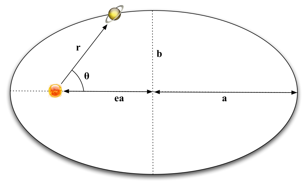
Fig. 48 Planetary orbits: an ellipse with the Sun at a focus.

Ellipse with Sun at one focus

Derived from Brahe’s observations of the orbit of Mars, this observation is a very useful result in orbital theory. Although we won’t use them much in this course, where we will mostly consider circular orbits, a few properties of ellipses are summarised here. An ellipse has semi-major axis \(a\), semi-minor axis \(b\) and eccentricity \(e\). An ellipse has two foci - each focus of an ellipse is a distance \(ae\) from the centre. A circle is a special case of an ellipse with \(e=0\); the focii of a circle are in the centre of the circle. The size of the semi-minor axis \(b\), the semi-major axis \(a\) and the eccentricity \(e\) are related by

\[b^2 = a^2 (1 - e^2).\]

Although the equation of an ellipse can be written in Cartesian co-ordinates (\(x\),\(y\)) it is more useful to use polar co-ordinates with a focus at the origin (as in figure 48). In this case, the equation of an ellipse is given by

(35)\[r = \frac{a(1-e^2)}{1 \pm e\cos\theta}.\]

At closest approach, the distance between a planet and the Sun is \(r_{p} = a(1-e)\), known as perihelion from the ancient greek ’peri’ (near) and ’helios’ (the Sun), while the furthest distance \(r_{a} = a(1+e)\) is known as aphelion since ’apo’ means away. In the case of the Moon orbiting the Earth, these are known as perigee and apogee, or periastron/apastron for planets orbiting other stars.

The 2nd Law

“For any planet the radius vector sweeps out equal areas in equal times”

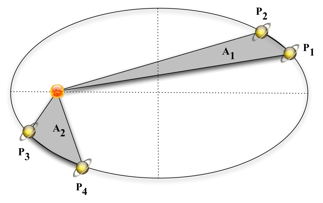
Fig. 49 Kepler’s 2nd Law.

Kepler’s second law

Kepler’s 2nd law is illustrated in figure 49. A1 is the area swept out as the planet moves from P1 to P2. A2 is the area swept out as the planet moves from P3 to P4. If the time taken to go from P1 to P2 equals the time taken to go from P3 to P4, then A1 equals A2. Just from looking at figure 49, you should be able to see that this means a planet will move faster when it is closer to the Sun.

The 3rd Law

“The cubes of the semi-major axes of the planetary orbits are proportional to the squares of the planetary periods”

Kepler’s 3rd law is a bit of a mouthful, but is more succinctly expressed in equation form,

(36)\[a^3 \propto P^2.\]

It turns out Kepler’s third law is incredibly useful, and we will use it again and again in this section of the course. Because of that, we really need to work out the constant of proportionality in equation (36) above. To do so, we need a full theory of gravity.

Newton’s law of gravity

On the 5th July 1687, Isaac Newton published his “Philosophi  Naturalis Principia Mathematica”. In it he set himself the incredible task of writing down the laws which governed the behaviour of everything in the Universe, from the smallest mote of dust to the planets themselves. It took him just three sentences:

• A body continues in a state of rest or uniform motion in a straight line unless compelled by some external force to act otherwise;

• The net force on an object is equal to the mass of the object multiplied by its acceleration;

• When a first body exerts a force on a second body, the second body exerts a force on the first body which is equal in magnitude and opposite in direction.

In the Principia, Newton also produced a derivation of Kepler’s laws from first principles. Since the planets are not moving in a straight line, some force must act upon them. Newton was able to show that his force of gravity reproduced Kepler’s laws in full. Newton’s gravitation force was, of course

(37)\[F = \frac{G m_1 m_2}{r^2},\]

where \(m_1\) and \(m_2\) are the masses of the two attracting bodies, and \(r\) is the distance between them. \(G = 6.673 \times 10^{-11}\)  m³ kg^-1 s^-2 is the gravitational constant.

It’s worth mentioning here that gravity is a tremendously weak force. The electrostatic repulsion between two protons is \(e^2/4\pi \epsilon_0 r^2\), whilst the gravitational attraction between them is \(Gm_p^2/r^2\). The ratio of these two quantities is \(e^2/4\pi \epsilon_0 G m_p^2\). This expression is independent of radius, so the relative strengths of the forces is the same throughout all space. The value of this expression is ! The electrostatic force is times stronger everywhere than the force of gravity, and yet it is gravity, not electromagnetism, that controls the motions of the stars and planets. This is because matter is mostly neutral. Large amounts of matter have negligible net charge, but very large masses; allowing gravity to become the dominant force.

An understanding of gravity is an incredibly versatile tool for an astrophysicist because it can be used to measure a basic property that, so far, we have no way of measuring; mass. By manipulating the laws of gravity we can make observations that allow us to measure the mass of astronomical objects as small as tiny satellites of Jupiter and as large as giant clusters of galaxies. To do so however, we need to spend a little bit of time developing some tools to use later in the course.

Proof of Kepler’s Laws

Before we proceed, lets work through a formal proof of Kepler’s Laws using vector calculus. First, we’ll need to consider conservation of angular momentum under gravity.

Conservation of Angular Momentum

To avoid over complication, lets assume that the star S is so much heavier than the planet P that we can consider it to be at rest. The angular momentum \(\vec{L}\) of P about S is the vector product \(m \vec{r} \times \vec{v}\), where \(m\) is the mass of P, \(\vec{r}\) is its position vector with respect to S and \(\vec{v}\) is its velocity. If we differentiate this with respect to time, using the product rule we get

\[\frac{d\vec{L}}{dt} = \left( m \frac{d\vec{r}}{dt} \times \vec{v} \right) + \left( m\vec{r} \times \frac{d\vec{v}}{dt} \right) = m\vec{v} \times \vec{v} + \vec{r} \times \vec{F}\]

where \(\vec{F}\) is the gravitational force on P due to S. Now the vector product of two parallel vectors is zero. Obviously \(\vec{v}\) is parallel to itself and \(\vec{F}\) acts along \(\vec{r}\) so both of the above vector products are zero. Therefore \(d\vec{L}/dt\) = 0, i.e. angular momentum is conserved under gravity.

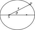
Fig. 50 Illustration showing the elliptical orbit of planet P around star S expressed as a vector in polar coordinates \(r\) and θ. Elliptical orbit in polar coordinates

To find the value of \(\vec{L}\), let us write the vector \(\vec{r}\) joining S and P as a vector in polar coordinates \(r\) and θ (figure 50),

\[\vec{r} = (r\cos \theta, r\sin \theta, 0).\]

Differentiate this, using the product rule (since both \(r\) and θ change with time), to give the velocity

\[\vec{v} = \left( \frac{dr}{dt}\cos \theta - r\frac{d\theta}{dt} \sin \theta, \frac{dr}{dt}\sin \theta + r\frac{d\theta}{dt} \cos \theta, 0\right).\]

Then the angular momentum \(\vec{L}\) is given by Note that this is exactly the same expression as we would get by considering circular motion, \(v = r\omega\), and writing the angular momentum as \(mvr\). This is sensible, as circular motion is just the special case in which \(r\) and ω are fixed. The difference is that this result holds even if \(r\) and ω are changing with time, providing the force between S and P acts along the line joining S and P.

Proof of Kepler’s 1st Law

Let us apply Newton’s second law, force = mass × acceleration, to the motion of P. As this is an ellipse, we need to consider both the usual circular motion acceleration \(\omega^2 r\), where ω is the angular velocity, and the rate of change of the distance \(r\) between S and P, so the acceleration has two components

\[\frac{-GM}{r^2} = \frac{d^2 r}{dt^2} - \omega^2 r.\]

We know from the previous section that \(\omega = L/(m r^2)\), so we can write this as

(38)\[\frac{d^2 r}{d t^2} = \frac{L^2}{m^2 r^3} - \frac{GM}{r^2},\]

which is a differential equation for \(r(t)\), where \(M\) is the mass of the star S. This can be simplified by making two changes of variable (one of these is not at all obvious!). Firstly, \(\omega = d\theta/dt\) we know that

\[\frac{d\theta}{dt} = \frac{L}{mr^2}\]

so by the chain rule

\[\frac{d}{dt} = \frac{d\theta}{dt} \frac{d}{d\theta} = \frac{L}{mr^2} \frac{d}{d\theta}.\]

Secondly, we change variable to \(u = 1/r\), so

\[\frac{dr}{dt} = \frac{d}{dt}\left(\frac{1}{u}\right) = -\frac{1}{u^2}\frac{du}{dt} = -\frac{L}{m}\frac{du}{d\theta}\]

and

\[\frac{d^2 r}{dt^2} = \frac{d}{dt} \left(\frac{dr}{dt}\right) = \frac{Lu^2}{m}\frac{d}{d\theta} \left( \frac{-L}{m} \frac{du}{d\theta}\right) = -\frac{Lu^2}{m^2} \frac{d^2 u}{d\theta^2},\]

using the result from above. If we substitute this into Equation (38) it becomes

\[-\frac{L^2 u^2}{m^2} \frac{d^2 u}{d\theta^2} = \frac{L^2 u^3}{m^2} - GM u^2.\]

dividing through by \(-L^2 u^2/m^2\) gives us

\[\frac{d^2 u}{d\theta^2} + u = \frac{GMm^2}{L^2}.\]

The solution to \(d^2 u/d\theta^2 + u = 0\) is just \(u = A \cos \theta\) (simple harmonic motion!), and it is easy to see that if we want \(d^2 u/d\theta^2 + u = k\), where \(k\) is a constant, we just add \(k\) to \(u\), so the solution to this equation is

\[u = \frac{1}{r} = A \cos \theta + \frac{G M m^2}{L^2}.\]

Recalling Equation (35), these are equivalent if

\[a(1-e^2) = \frac{L^2}{GMm^2}\]

and

\[e = \frac{A L^2}{G M m^2}.\]

Note that \(A\) is an arbitrary integration constant. Therefore the value of \(a(1-e^2)\) is fixed by physical constants, namely the angular momentum of the planet and the mass of the star, but the eccentricity is arbitrary. An eccentricity of 0 gives a circular orbit. Finally, note that because \(L \propto m\), the characteristics of the orbit don’t really depend on the planet’s mass, providing it is small enough that we can neglect the motion of the star. The real physical variable is the specific angular momentum, i.e. the angular momentum per unit mass, usually given by the symbol \(\vec{h}\) (as a vector) or \(h\) (its magnitude - not to be confused with Planck’s constant!).

Proof of Kepler’s 2nd Law

Consider a small area, \(dA\), of the ellipse swept out in time \(dt\), represented by the triangle in Figure 51,

\[dA = \frac{1}{2} \times (r + dr) \times r \sin (d\theta).\]

Since both \(dr\) and \(d\theta\) are small, we can use the small angle approximation \(\sin (d\theta) \simeq d\theta\), and neglect any terms involving \(dr \times d\theta\), so

\[\frac{dA}{dt} \simeq \frac{1}{2} r^2 \frac{d\theta}{dt} = \frac{1}{2} r^2 \omega = \frac{h}{2}\]

where \(h\) is the specific angular momentum defined above. We know that both \(\vec{L}\) and \(m\) are constants, so it follows that \(h = L/m\) is also constant. Therefore \(dA/dt\), the rate at which the radius vector sweeps out area, is also a constant.

Fig. 51 Illustration showing the area of an ellipse swept out in time \(dt\).

Area of an ellipse swept out in unit time

It can be shown that the orbital velocity at perihelion, \(v_{p}\), can be written as

\[v_{p} = \frac{2 \pi a}{P} \left( \frac{1+e}{1-e} \right)^{0.5}\]

while the orbital velocity at aphelion, \(v_{a}\), is

\[v_{a} = \frac{2 \pi a}{P} \left( \frac{1-e}{1+e} \right)^{0.5}\]

so

\[\frac{v_{p}}{v_{a}} = \frac{1+e}{1-e}.\]

More generally,

\[v^2 = GM \left(\frac{2}{r} - \frac{1}{a}\right).\]

Further details are provided in Section 3 of the Celestial Mechanics chapter in the Carroll & Ostlie textbook. For small eccentricies, \(v_{p} \sim 2\pi r_{a}/P\) and \(v_{a} \sim 2\pi r_{p}/P\), since \(r_{a} = a (1+e)\) and \(r_{p} = a (1-e)\).

Proof of Kepler’s 3rd Law

The area of an ellipse is \(\pi ab\), the rate at which area is swept out \(dA/dt = h/2\), so the period \(P\) (the time taken to sweep out the whole area) is

\[P = \frac{2\pi ab}{h} = 2\pi a^2 \frac{\sqrt(1-e^2)}{h}.\]

Squaring this, and substituting in \(h^2 = GMa(1-e^2)\) from earlier, we get

(39)\[P^2 = \frac{4 \pi^2 a^4 (1-e^2)}{GMa (1-e^2)} = \frac{4 \pi^2}{GM} a^3.\]

This gives us \(P^2 \propto a^3\), as required, and also tells us what the constant of proportionality is.

If we measure the star’s mass in units of the Sun’s mass, the semi-major axis in astronomical units, and the period in years, the constant \(4\pi^2/G\) must be numerically equal to 1, because for the Earth we get \(1^2 = 1^3 \times 4 \pi^2 / (1 \times G)\). This can be useful in some numerical problems. For example, the highly eccentric (\(e\) = 0.84) orbit of the Kuiper Belt Object Sedna has a semi-major axis of \(a\)=480 AU, so because \(M = M_{\odot}\), its orbital period is \(P\)/yr = (\(a\)/AU)\(^{3/2}\) or 10,500 yr!

Circular orbits

For the remainder of the course we will limit our discussion to circular orbits. We will derive some very useful results which follow from Newton’s law of gravity. We will need these results later on in the course, but let’s revisit Kepler’s 3rd law once again and show that it too can be also derived from Newton’s law of gravity.

Kepler’s 3rd law revisited

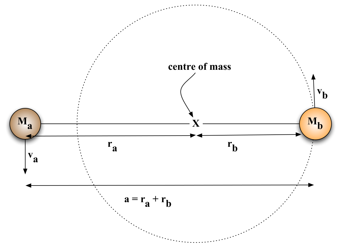
Fig. 52 Circular orbits around the centre of mass (CoM). The centre of mass is marked with a cross, whilst the circular orbit of star b around the CoM is shown as a dotted line.

Circular orbits of two stars around their centre of mass

In the Solar system, Kepler stated that the planets orbit around the Sun. This is because the Sun is much heavier than the planets. In the general case of two bodies orbiting under their mutual gravitational attraction, both bodies perform circular orbits around the centre of mass. This situation is shown in figure 52.

We can derive Kepler’s third law by equating force and mass × acceleration. The acceleration of an object in a circular orbit is \(v^2/r\), so for star b (using the notation from figure 52),

\[\frac{GM_aM_b}{a^2} = \frac{M_bv_b^2}{r_b}.\]

Similarly, for star a,

\[\frac{GM_aM_b}{a^2} = \frac{M_av_a^2}{r_a}.\]

Adding these two, we find

\[\frac{G(M_a+M_b)}{a^2} = \left( \frac{v_a^2}{r_a} + \frac{v_b^2}{r_b} \right).\]

Now, we use one of the neat mathematical tricks that crop up throughout gravitational astrophysics. The distance round a circular orbit of radius \(r\) is \(2\pi r\), and the time taken to go round the orbit is \(P\). Therefore, we can write

\[v = \frac{2\pi r}{P},\]

and substitute this into our equation above to get

\[\frac{G(M_a+M_b)}{a^2} = \left( \frac{4\pi^2 r_a}{P^2} + \frac{4\pi^2 r_b}{P^2} \right) = \frac{4\pi^2}{P^2} (r_a + r_b) = \frac{4\pi^2}{P^2} a.\]

Re-arranging, we find

(40)\[\frac{GP^2(M_a+M_b)}{4\pi^2} = a^3,\]

which you can see is identical to equation (39) with \(M = M_{a} + M_{b}\). The form of Kepler’s third law shown in equation (40) crops up again and again. It is worth spending some time memorising it.

Gravitational potential energy

It is useful to define the gravitational potential energy; the work required to separate two bodies to an infinite distance from an initial separation \(r\). We start by asking how much work is required to move them a small distance \(dr\). Since work = force × distance

\[\text{Work} = -\frac{Gm_1m_2}{r^2} dr\]

Why the minus sign? Because the direction of the force and \(dr\) are in opposite directions. If we choose our radius axis so that \(dr\) is positive, then the gravitational force is \(-Gm_1m_2/r^2\). The total work moving the bodies to infinity is the sum of all the little steps along the way

(41)\[\text{Grav. P.E} = -\int_r^\infty \frac{Gm_1m_2}{r^2} dr = \left[ \frac{Gm_1m_2}{r} \right]_r^\infty = -\frac{Gm_1m_2}{r}.\]

This quantity is negative; as expected because we have to put energy in to separate the two bodies. The gravitational potential energy leads to the concept of escape velocity. One object will escape the gravitational field of another if its kinetic energy is larger than the size of the gravitational potential well,

(42)\[\frac{1}{2} m_2v^2 > \frac{Gm_1m_2}{r} = v _{esc} > \left( \frac{2Gm_1}{r} \right)^\frac{1}{2}\]

Gravitational theorem #1

“A body inside a spherical shell of matter experiences no net gravitational force from that shell”

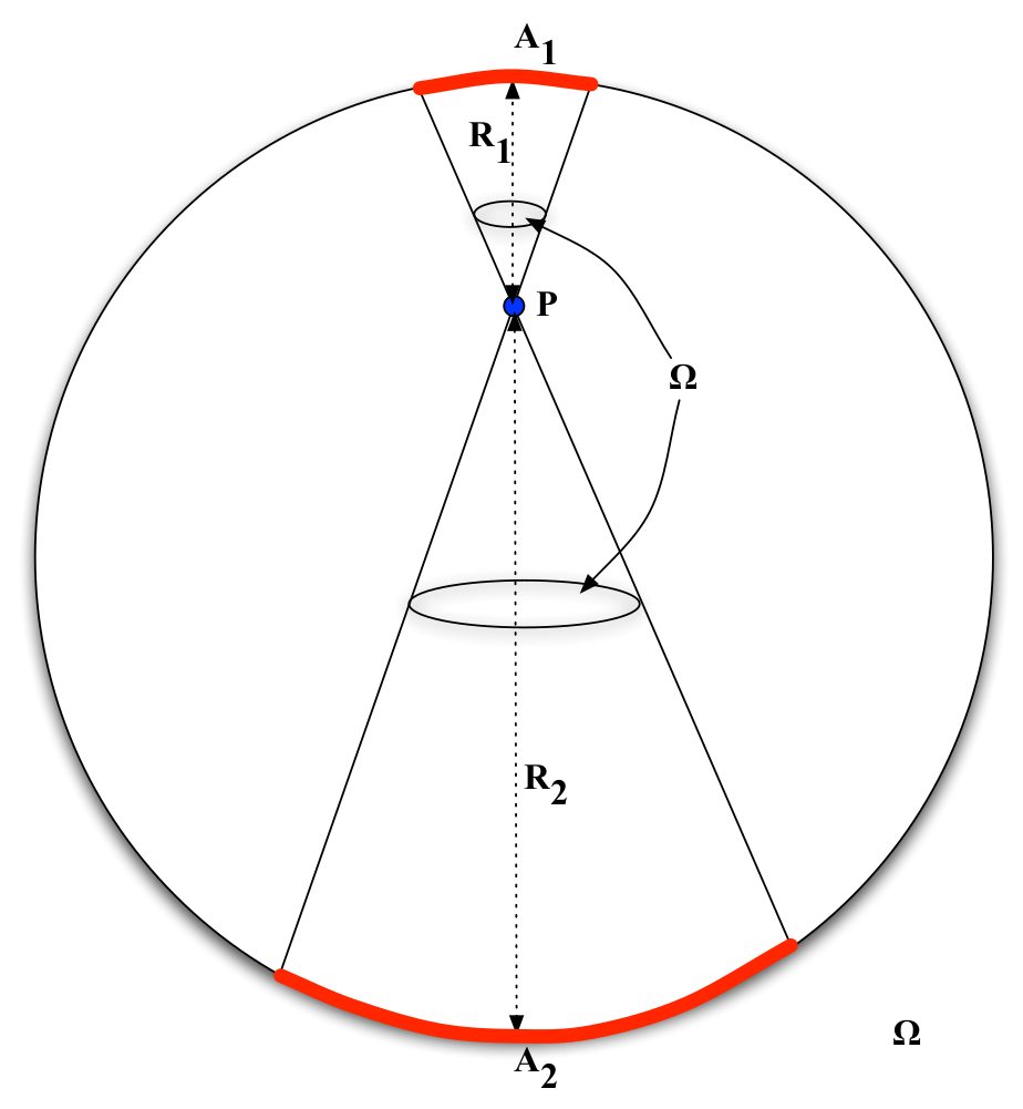
Fig. 53 A point P inside a hollow, thin shell experiences no net gravitational force.

No net gravitational force inside a hollow thin shell

This turns out to be OK to derive. We imagine the shell to be thin, with a density of ρ kg per unit surface area. We pick a point, \(P\) inside the shell and draw two cones of the same solid angle radiating out from the point \(P\), so that they includes two small areas of the shell on opposite sides: these two areas will exert gravitational attraction on a mass at \(P\) in opposite directions. We will show that these forces exactly cancel out. The situation is shown in figure 53.

Since the cones have the same solid angle Ω, and the area of the base of a cone of solid angle Ω is \(A = \Omega r^2\), we see that the ratio of the areas \(A_1\) and \(A_2\) at distances \(r_1\) and \(r_2\) are given by \(A_1/A_2 = r_1^2/r_2^2\). Since the masses of the bits of the shell are proportional to the areas, the ratio of the masses of the shell sections is also \(r_1^2/r_2^2\). It follows that the ratio of the gravitational forces from the two bits of shell is

\[F_1/F_2 = \frac{M_1}{M_2} \frac{r_2^2}{r_1^2} = \frac{r_1^2}{r_2^2} \frac{r_2^2}{r_1^2} = 1.\]

So the forces on a particle at \(P\) due to these sections of shell are the same size and in opposite directions; they cancel exactly. In fact, the gravitational pull from every small part of the shell is balanced by a part on the opposite side?ou just have to construct a lot of cones going through \(P\) to see this. So the net force on a particle inside the shell is zero.

What if the shell is not thin? A particle inside a spherical cavity in a dust cloud is such a situation. We can consider it as an infinite number of thin shells nested inside each other. The force from each shell is zero, so the net force inside a cavity like this is also zero. This result will be tremendously important when we look at measuring mass in galaxies.

Gravitational theorem #2

“The gravitational force on a body that lies outside a closed spherical shell of matter is the same as it would be if all the shell’s matter were concentrated into a point at it’s centre.”

We’ve already assumed that this theorem is true, when we derived Kepler’s 3rd law; we implicitly assumed we could treat the stars as point masses, even though they are spheres of finite size. There is a beautiful and elegant proof of this theorem, which can be written in about three lines, using a different way of writing the law of gravity known as Gauss’s theorem. Unfortunately for you, the maths used is (I believe) more advanced than you have learned to date. By contrast, Newton’s derivation took him several pages to write and years to figure out! Therefore we will take this theorem to be true without proof; the curious will find complete derivations using Newton’s method or the Shell theorem. Gauss’s theorem is really quite beautiful mathematics, and allows you to easily work out the gravity from complex objects.