
Chapter 5: Thermal Continuum Radiation#
The colours of stars#
Thermal continuum radiation#
In everyday life, most objects are visible because of the light which they reflect. You and I are visible because of the sunlight we reflect, not because of the light we emit ourselves. We do, however, emit light. All material objects give of some radiation: the hotter they are, the more radiation they emit. Can we be more specific about the properties of light emitted by warm objects?
We can if we make one very important approximation; that the radiation emitted by an object is in thermal equilibrium with it’s surroundings. What do we mean by that? Suppose we heat an object up; it will radiate light. This radiation carries away energy and so the object cools. Now, we’ll put our object into a special box, which absorbs and re-emits all of the radiation which falls upon it. Now, as our object cools, the box fills with photons. Some of these will be absorbed by our object, and provide a small heating effect. Eventually, a balance will be set up, where for every photon absorbed another is emitted by the object. At this point the box, the radiation and the object are all in thermal equilibrium. This is a stable situation; the spectrum of the radiation does not change with time. The radiation within the box is called thermal equilibrium radiation. It is often called black-body radiation, because the best way to get the box walls to absorb and emit all the radiation is to make them black.
Suppose we now make a tiny, tiny hole in the box. Just large enough to allow some light to escape, but not so large as to break the thermal equilibrium within the box. What does the spectrum of the light look like?
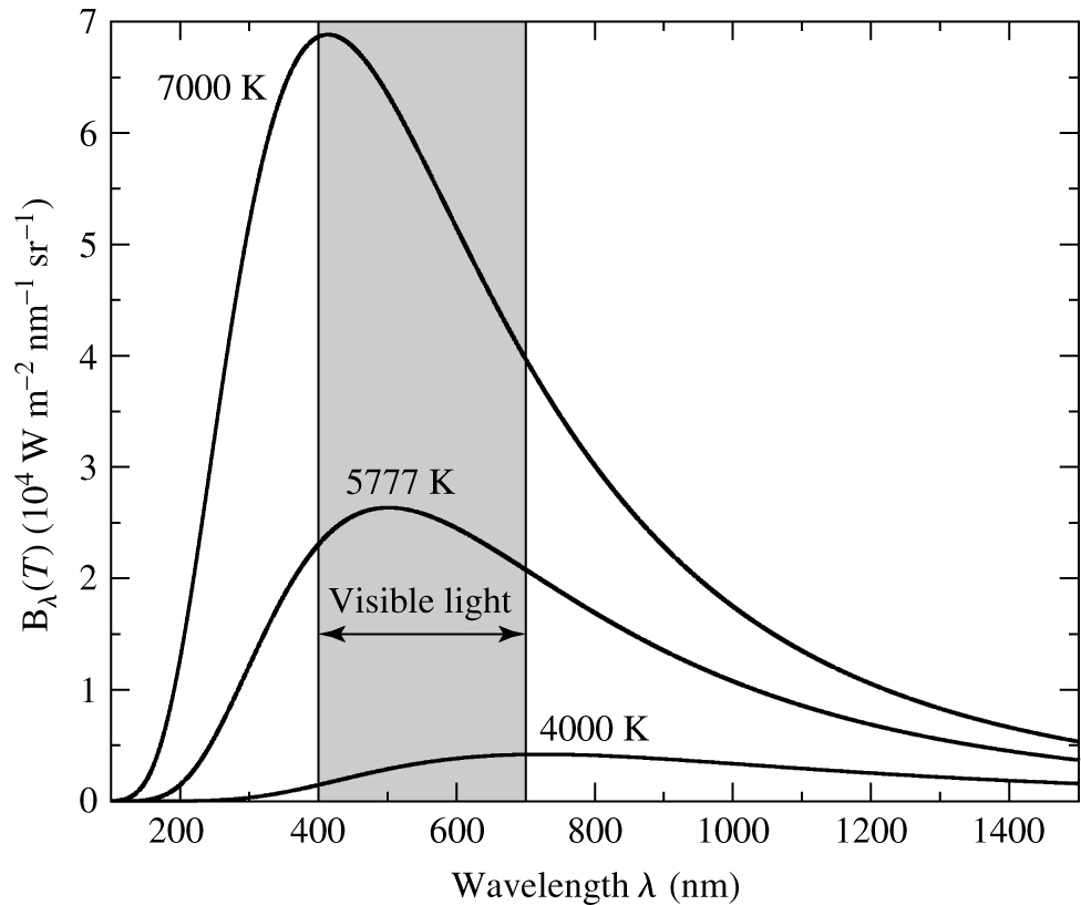
Fig. 18 Black body light curves. Monochromatic intensity (monochromatic flux per unit solid angle) is plotted against wavelength for black bodies at three temperatures. The wavelength range of visible light is shown.#
Blackbody curves
Black-body spectra for objects at three temperatures are shown in figure 18. The curves show a steep rise to a well-defined peak, and then a tail of emission towards longer wavelengths. As the temperature increases, the peak moves to shorter wavelengths, and the area under the curve increases. A derivation of the formula which describes the black-body spectrum is not easy, and produced the first quantum mechanical formula ever known. The German physicist, Max Planck, first determined the formula empirically, by fitting the observed curve with a function that gave an extremely good fit. Classical physics was completely unable to explain why this formula worked so well, but quantum mechanics provided the answer. The formula, now known as the Planck function is
\(B_{\nu}(T)\) is the monochromatic surface flux. It is still the amount of light per unit time, per unit frequency and per unit area, but now that unit area refers to a small unit of area on the surface of the emitting object. The Planck function is extremely important in astrophysics, and we shall examine some of the implications of it in the next lecture. But before we do; what objects actually emit as black bodies?
Black bodies in Astrophysics#
The pedantic answer to the question above is that nothing emits as a black body. Perfect thermal equilibrium is impossible to achieve. However, there are important classes of object that are very nearly in thermal equilibrium, and so emit roughly as black bodies. What properties does an object need to be close to thermal equilibrium? It must be a near perfect absorber of light, or else it will reflect and the spectrum will differ from a black body. Also, since it absorbs perfectly, it must also emit perfectly, or else it will steadily absorb energy and heat up. Obviously, the object needs to have a stable temperature (it needs to be in thermal equilibrium).
A good example is dust grains. Dust grains are bathed in radiation from the surrounding stars. Moreover, they are good absorbers and emitters. Therefore, they quickly reach a temperature where the radiation emitted from the grains balances that absorbed from the background starlight. Another good example is the Cosmic Microwave Background. This background radiation emitted at a time when the Universe was small, hot and opaque, is almost a perfect black-body. It has cooled as the Universe has expanded, and has a black-body spectrum corresponding to a temperature of 2.725K (see figure 19).
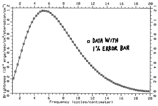
Fig. 19 Cosmic Microwave Background spectrum as measured by COBE. The theoretical curve is the Planck function for a 2.725K black body.#
Cosmic Microwave Background
However, the most important example of black bodies in astrophysics are stars themselves. Since the energy lost through radiation is balanced by heat from nuclear fusion in their cores, stars have a stable temperature. And they are so dense in their interiors that nearly every photon is absorbed (they are very good absorbers and re-emitters). However, stars are not perfect black bodies. This is because the outer layers of the star is not a perfect absorber/emitter of radiation. Instead, near the surface of the star, the absorption of light is a strong function of wavelength. Starlight is therefore only approximated by the Planck curve.
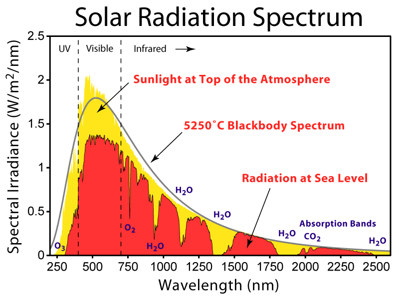
Fig. 20 Monochromatic flux from the Sun, as observed at ground level (red) and after correction for the absorption by the atmosphere (yellow). The spectrum is reasonably well fit by a black body curve for a temperature of 5250 K.#
Solar Spectrum
Figure 20 shows the Solar spectrum. After correction for the absorption by the atmosphere, the Sun’s spectrum is pretty closely predicted by the Planck function, but the agreement is not perfect. The fact that we can, to a rough approximation, treat stars as black bodies allows us to make many important deductions about their properties.
Blackbody radiation in wavelength units#
Eqn. (10) is the formula for the spectrum of blackbody radiation in frequency units. It is a monochromatic surface flux, so it gives the energy emitted per unit surface area, per unit time and per unit frequency. What is the corresponding curve in wavelength units? You might remember we solve this question by realising that the amount of energy emitted in a small frequency range must equal the amount of energy contained within the corresponding wavelength range, \(F_{\nu}d\nu = F_{\lambda} d{\lambda}\). That lead to equation (3),
We can now use that equation to write the Planck curve in wavelength units
We now substitute in \(\nu = \frac{c}{\lambda}\) into the equation above to obtain
Wien’s Law#
At what wavelength does a hot body emit the most light? Assuming the hot object is roughly a black body, this question boils down to finding out at what wavelength the Planck curve peaks. The calculation is simple in principle, and a bit complicated in practice. In principle, we find the maximum (or minimum) of a function by finding where the derivative is zero. In other words, the peak wavelength, \(\lambda_{peak}\) is the one which satisfies
The solution to this equation is not so straightforward. I’m going to include (most of) it here, because it serves as a useful example of how to solve a complex differentiation problem. The derivation is non-examinable, however, and so the truly math-phobic might want to skip to the answer.
The derivation#
We want to solve
We make a start by writing \(B_{\lambda}(T) = uv\), where
From the product rule, \(\frac{dB}{d\lambda} = u\frac{dv}{d\lambda} + v\frac{du}{d\lambda}\). First, we calculate \(v\frac{du}{d\lambda}\) easily
Next, we calculate \(u\frac{dv}{d\lambda}\). This is a little harder.
We can’t easily do the differential in the square brackets, so we try to apply a few standard tricks to make it easier. In this case, we make a substitution \(x=\frac{hc}{\lambda kT}\).
and use the product rule
. Since \(x=\frac{hc}{\lambda kT}\),
Substituting this in to our earlier equation, we find
But we still can’t simply write the answer for the differential in the formula above. However, we are now very close, because we can apply the quotient rule,
and set \(f(x) = 1\), and \(g(x) = e^x -1\). It follows that \(df/dx = 0\) and \(dg/dx = e^x\). If we use this, we find
So now we have,
Phew! So now going back to \(\frac{dB(T)}{d\lambda} = u\frac{dv}{d\lambda} + v\frac{du}{d\lambda}=0\), we find
The term outside the square bracket in that equation is always positive, and never zero. That means the term inside the square brackets should be zero and so we arrive at…
Unfortunately the answer we’ve reached is not very useful. We can’t use it to find the value of the wavelength at the peak of the black body function yet. Worse, it is fiendishly difficult (though possible) to solve this equation analytically. Instead, we can use a computer to solve it numerically, in which case we arrive at…
The answer#
We can make this answer even more memorable by re-arranging, and substituting in S.I values for \(h\) and \(c\), to get
where the wavelength is measured in metres, and the temperature in Kelvin. This formula is known as Wien’s Law, after Wilhem Wien, who derived it (following a different line of argument) in 1893. It shows that the peak wavelength of the Planck curve is inversely proportional to temperature. We have derived the property discussed last lecture that as the temperature of a body increases, the peak wavelength gets shorter (see figure 18).
At a room temperature of \(\sim290\) K, \(\lambda_{peak}\) is about 10 microns. This is well into the infrared spectrum of light, and our eyes are not sensitive to these wavelengths. This explains why we see objects only from the sunlight they reflect and scatter. If our eyes were sensitive to infrared light, we would see the thermal radiation from everyday objects, like in figure 21.
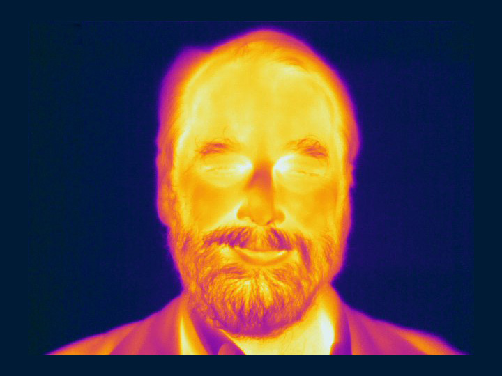
Fig. 21 An image taken at a wavelength of 12 microns of Prof Ned Wright (Caltech). Prof Wright is the lead scientist on NASA’s WISE mission, which has surveyed the night sky at infrared wavelengths between 3 and 12 microns. These wavelengths are not accessible from Earth, because the water vapour in the atmosphere makes it opaque (recall Fig. 6).#
Prof Ned Wright at 12 microns
Our Sun, has a temperature around 5800 K. Using Wien’s law, the Sun’s spectrum peaks at about 0.5 microns. It is by no means a coincidence that this is close to the middle of the range of light to which our eyes are sensitive! The middle curve in figure 18 is a decent approximation to the Sun’s spectrum. You’ll notice that the sun emits light more or less evenly across the whole visual range. Sunlight is thus a pretty even mix of colours, and we perceive it as white. However, the sunlight which reaches the Earth has passed through the atmosphere. Since the atmosphere preferentially scatters blue light most of the blue part of the Sun’s spectrum is scattered. That is why the Sun looks yellow, and the sky looks blue.
Colours and colour temperature#
In principle, Wien’s Law gives us a way to obtain a measurement of stellar temperature. In practice we often don’t have sufficient data to measure the peak wavelength accurately. However, we can easily measure the colours of stars, and since Wien’s law tells us that objects get bluer as they get hotter, it shouldn’t be a surprise that the colour of a star can provide a measure of the temperature.
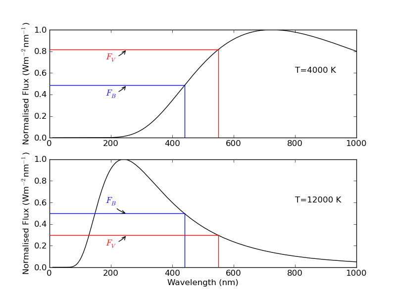
Fig. 22 Colour indices and temperature. The top panel shows a black body at a temperature of 4000 K, and the bottom panel shows a black body at a temperature of 12,000 K. Clearly, the ratio of B-band flux to V-band flux increases with increasing temperature. On our magnitude scale, that corresponds to a \(B-V\) colour index which decreases with increasing temperature.#
Colour indices and temperature
The colour index, which we defined in equation (5), was the difference in magnitude, as measured in two filters, e.g.
Using the Planck curve, we can see that the colour index is a direct measure of temperature. Figure 22 shows two blackbodies, one at 4,000 K and another at 12,000 K. The 4,000 K blackbody emits less light at \(B\) than at \(V\), and so it’s \(B-V\) colour index is positive. By contrast, the 12000 K blackbody emits more light at \(B\) than at \(V\), and so it’s \(B-V\) colour index is negative. Thus, we see that \(B-V\) gets smaller as the star gets hotter and bluer.
We can get a temperature estimate directly from a star’s \(B-V\) colour. We simply ask what black body curve would show the same \(B-V\) colour as we observe. Temperatures derived in this manner are called colour temperatures. Of course, since the star is not a perfect black body, the colour temperature is only an approximation to the star’s true temperature.
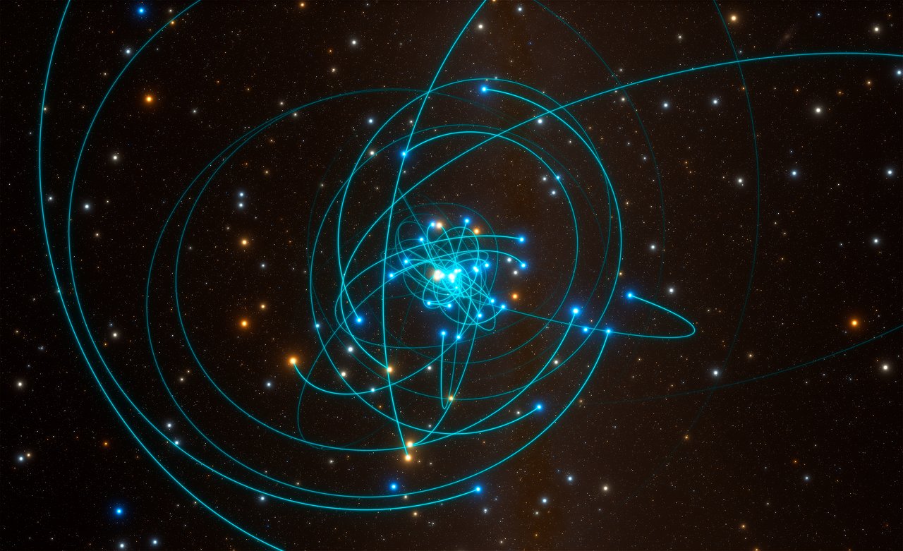
Fig. 23 Orbits of stars around the supermassive black hole Sgr A* at the centre of the Milky Way. Monitoring is performed in the near infrared since extreme dust extinction towards the Galactic Centre prevents observations at shorter wavelengths. Credir: ESO/L. Calcada/spaceengine.org#
Motion of stars around Sgr A star
There is one additional complication that we haven’t touched on so far, which is interstellar dust. Dust comprises sub-micron sized particles which absorb light, especially at optical and ultraviolet wavelengths, and makes up typically 1% of the mass of interstellar matter (interstellar gas makes up the remaining 99%). The volume density of dust is low in the interstellar medium, so nearby objects (parsec distances) are relatively unaffected, but distant object in the disk of the Milky Way are affected, and appear redder than they would without interstellar dust, since dust preferentially absorbs shorter wavelengths. Consequently we need to allow for dust if calculating a colour temperature from \(B - V\). If the intrinsic colour of a star is \((B - V)_{0}\), and the observed colour is \(B - V\), then the difference, or colour excess \(E(B - V)\) is
so colour temperatures will only be practical for nearby stars unaffected by interstellar extinction. The amount of visual extinction, \(A_{\rm V}\), is approximately
and can be substantial for objects located several kiloparsec away in the disk of the Milky Way (\(A_{\rm V} \sim 1-2\)/kpc). Indeed, the effect is colossal in extreme cases, such as the Galactic Centre where \(A_{\rm V} \sim 30\) mag, so individual sources appear 1012 times fainter in the visible than they would otherwise. Consequently, observations of the Galactic Centre are not feasible at optical wavelengths, so have to be carried out at infrared or radio wavelengths where the dust absorption is much lower. Time lapse images of stars in the Galactic Centre orbiting the central supermassive black hole, Sagittarius A* – Andrea Ghez and Reinhard Genzel were jointly awarded the 2020 Nobel Prize in Physics for their observations of Sgr A* – are usually obtained in the near-infrared K-band window at 2μm, since \(A_{\rm K} \sim 0.1 \times A_{\rm V} \sim\) 3 mag, so individual stars appear (only) 15 times fainter than they would in the absence of interstellar dust (Fig. 23).
Therefore, Equation (7) which connects apparent magnitude, \(m_{\lambda}\), absolute magnitude \(M_{\lambda}\), and distance \(d\) becomes
taking interstellar extinction \(A_{\lambda}\) into account, although extinction can safely be neglected for stars within the Solar Neighbourhood (few hundred parsec).
The Stefan-Boltzmann Law#
Let’s use the Planck curve to work out another property of black bodies. What is the total flux emitted if we sum over all frequencies/wavelengths? In other words, what is the bolometric surface flux from a black body? To find this, we need to integrate the Planck curve over all frequencies (I’m going to use frequency here, rather than wavelength, because it makes the integration a bit easier). So, the bolometric surface flux is given by:
This is quite a hard integral, although it’s a lot easier than the derivation of Wien’s Law above. We’ll make it look a bit simpler by substituting \(x = \frac{h\nu}{kT}\), so \(\nu = \frac{xkT}{h}\) and \(d\nu = \frac{kT}{h} dx\):
If we tidy a few terms up, and take all the constant terms outside the integral, we get
The integral \(\int_0^\infty \frac{x^3}{e^x-1} dx\) is not trivial, but fortunately it can be looked up in a table of standard integrals. It’s value is simply a constant;
which we can substitute to get
This is the Stefan-Boltzmann equation. It shows that the bolometric surface flux from a black body is proportional to the temperature to the fourth power. The constant of proportionality in the equation above is called Stefan’s constant, and given the symbol σ. In this form, the Stefan-Boltzmann equation looks like
where \(\sigma = 5.67\times10^{-8}\) Wm-2K-4.
Flux and luminosity from black bodies#
The Stefan-Boltzmann law gives the bolometric surface flux from the black body. In otherwords, it is the total energy emitted at all frequencies, per second and per unit area of the black bodies surface. To find the total energy emitted per second from the black body, we need to multiply by the surface area of the black body, so
in Watts. We can use the inverse square law \(F=L/(4\pi d^2)\), to calculate the bolometric flux at a distance, \(d\) from the black body
in Watts per square metre.
Effective Temperatures and Bolometric Corrections#
Equation (13) can be used to estimate the surface temperature of a star. We measure the bolometric flux from Earth. Usually this involves measuring the monochromatic flux at as many wavelengths as possible, and integrating over them to obtain the bolometric flux. In many instances it is not possible to calculate the distance \(d\) to a star, but if we can measure its angular diameter (θ), the angular radius \(\theta/2 = R_{*}/d\) allows the temperature to be estimated, since Equation (13) is equivalent to
in Watts per sequare metre. Temperatures obtained this way are known as effective temperatures. They are the surface temperature the star would have if it radiated as a perfect black body. Again - since stars are not perfect black bodies - the effective temperature is only an approximation to the actual surface temperature of the star.
If both the effective temperature of a star and its distance is known, the absolute bolometric magnitude, \(M_{\rm Bol}\) can be expressed as
where \(M_{V}\) is the absolute visual magnitude and we have introduced the bolometric correction, \(BC\), which is a temperature-sensitive function. Bolometric corrections are small for stars which emit the bulk of their energy in the visual (\(BC = -0.08\) mag for the Sun), but corrections are large for blue and red stars alike, which emit primarily in the ultraviolet or infrared, respectively. One may convert between absolute bolometric magnitudes and luminosities as follows
since the absolute bolometric magnitude of the Sun is \(M_{\rm Bol}\) = +4.74 mag.
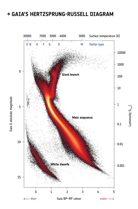
Fig. 24 Colour magnitude diagram for 4 million stars whose distances have been obtained from parallax measurements by the Gaia satellite. Acknowledgement: Gaia Data Processing and Analysis Consortium (DPAC); Carine Babusiaux, IPAG – Universit Grenoble Alpes, GEPI – Observatoire de Paris, France.#
Colour magnitude diagram from Gaia parallaxes
Fig. 24 reveals a colour magnitude diagram for 4 million stars observed with ESA’s Gaia satellite, from which distances were obtained from parallax measurements. Stars are plotted according their colour (horizontal axis) and brightness (vertical axis). Brighter stars are shown in the upper part of the diagram, with fainter stars at the bottom. Hotter, bluer stars are on the left, and cooler, redder stars on the right. Colours are used to indicate the density of stars in a particular region, such that the diagonal stripe across the centre of the graph is known as the main sequence, in which dwarf stars are undergoing core hydrogen burning. Giant red stars are shown in the upper right part of the diagram while white dwarfs, the remnants of low mass stars, are shown in the lower left. This is a huge improvement on Hipparcos, which was only able to obtain distances for tens of thousands of stars.
Other continuum emission mechanisms#
The thermal radiation emitted by hot objects is a continuum emission mechanism. By that we mean that the light emitted is spread out over a broad range of wavelengths, and has no sharp features in its spectrum. It is not the only continuum emission mechanism encountered in astrophysics, and for completeness I’ll briefly mention some of the other mechanisms here.
Synchrotron radiation#
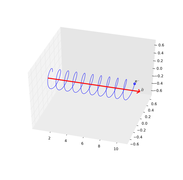
Fig. 25 Synchrotron radiation is produced by electrons spiralling around the magnetic field lines#
Synchrotron radiation
Synchrotron radiation is emitted by electrons which move at close to the speed of light, in the presence of strong magnetic fields. The electrons feel a force from the magnetic fields, which result in them spiralling around the field lines (Figure 25). Put another way, the electrons feel an acceleration from the magnetic field, and since all accelerated charges emit radiation, light is emitted from the electrons. Synchrotron radiation is emitted from regions where there are both fast moving electrons, and strong magnetic fields.
Synchrotron radiation has a characteristic power-law spectrum, given by
where \(n \sim\) 0.5–1.5. This means that most of the light emitted as synchrotron radiation is emitted at low frequencies (long wavelengths). Synchroton radiation is a source of radio waves, with wavelengths longer than a cm or so.
Bremsstrahlung#
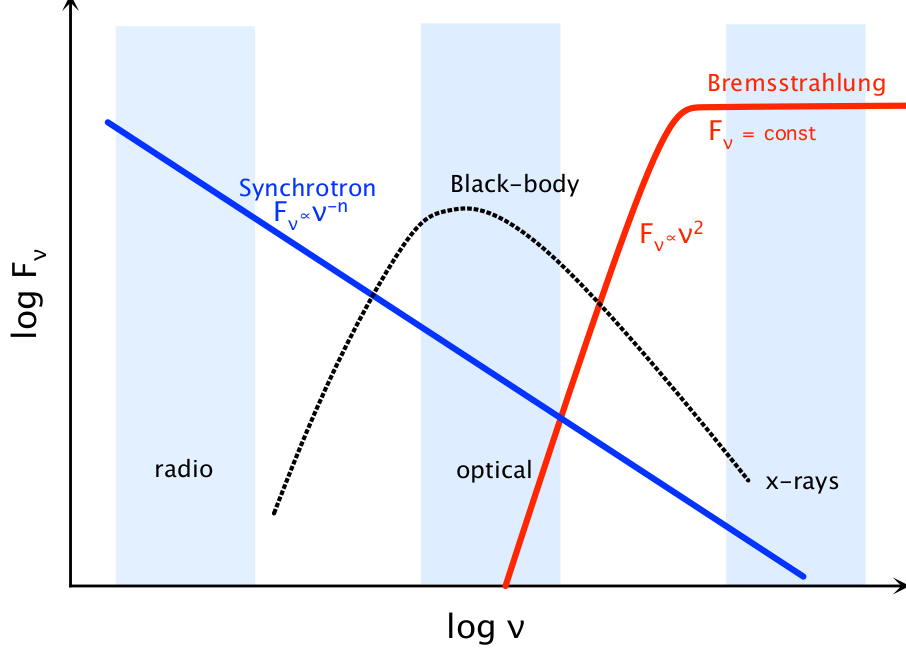
Fig. 26 A sketch of the contribution of various continuum sources at different frequencies#
Contributions from Synchrotron, thermal and Bremsstrahlung radiation
Bremsstrahlung or braking radiation is emitted from ionised gasses. As the electrons move past the protons, they feel an electric force, which decelerates them. Once, again, accelerated charged particles emit radiation, so the electrons emit light as they are braked. For the gas to be ionised it must be very hot, so that there is enough energy to free the electrons from atoms. It is not surprising that bremsstrahlung is mostly emitted at high frequencies. In fact, the spectrum from bremsstrahlung is flat; the amount of flux emitted is independent of wavelength. Below some cutoff wavelength, however, the flux is proportional to the square of the frequency, so very little light is emitted at low frequencies (the spectrum is sketched in figure 26.). The cutoff frequency is high; bremsstrahlung is a good source of X-rays.
Figure 26 also illustrate the point that the different continuum emission mechanisms produce light at very different wavelengths. As a result, the appearance of an astrophysical object can change drastically with wavelength. In the optical, we see thermal radiation from hot objects, like stars. The infrared is also dominated by thermal emission, but from cooler objects, like dust. At radio wavelengths, if an object has a strong magnetic field and can produce very fast moving electrons, we will see synchrotron radiation from those electrons. In the X-rays, we might see bremsstrahlung from hot gas, at least so long as there is sufficient ionised gas!