Chapter 8: The Bohr model of the atom

Chapter 8: The Bohr model of the atom#

The spectroscopic work carried out up till the beginning of the 20^th century has left us with three facts which need explaining:

the presence of discrete lines in the emission spectra of elements;
the Kirchhoff-Bunsen rules, which dictate what kind of spectrum will be observed from different sources
the nature of the Harvard Spectral Sequence

In this section, I will try and tackle the first two questions. The question we are really seeking to answer is how does an atom of, say, Hydrogen interact with light. Why does it emit and absorb at discrete wavelengths? To answer this question, we need to examine the structure of an atom.

The atom#

In the final years of the 19^th century, J.J Thomson discovered the electron. Since matter (and hence atoms) is neutral, this discovery meant that the atom consists of negatively charged electrons, and some distribution of positive charge. In 1911, Ernest Rutherford showed that the positive charge was confined to a tiny, massive nucleus. He did so by firing energetic alpha particles at thin metal foils. Astoundingly, some of the alpha particles bounced off the foil. Rutherford wrote:

“It was quite the most incredible event that has ever happened to me in my life. It was almost as incredible as if you fired a 15-inch shell at a piece of tissue paper and it came back and hit you.”

Rutherford’s work led to a picture of the atom in which negatively charged electrons orbited around a tiny, positively charged and massive nucleus. This atomic picture had two major flaws. Firstly, it was known from Maxwell’s theories of electromagnetism, that acclerating charges emit radiation. An electron in a circular orbit is constantly accelerating – Its speed may be constant, but its direction is constantly changing. This is because it feels the attractive force of the nucleus; it is this force that provides the acceleration – and so it should emit radiation, lose energy and spiral into the nucleus. This should all happen in less that s. Obviously matter is stable on very long timescales, so this is a major flaw in the model! Secondly, the atom as described couldn’t explain the work of Kirchhoff and Bunsen, who showed that atoms absorb and emit light at discrete wavelengths.

Niels Bohr and the ’semi-classical’ atom#

At the same time as Rutherford was beginning to understand the nature of the atom, theoretical physicists were beginning to grasp the quantised nature of light. Einstein’s work on the photoelectric effect showed that light existed as photons with quantised energy, and this idea was exploited by Max Planck, who used it to derive the Planck curve for Black Body emission.

The Danish physicist, Neils Bohr made a great step towards solving the structure of the atom by making a massive leap of intuition. Bohr noted that the dimensions of Planck’s constant [Js] are equivalent to [kg m² s^-1], the dimensions of angular momentum. What if the angular momentum of the electron was quantised? Just as an electron magnetic wave, made out of \(n\) photons fo frequency ν, could only have an energy of \(E=nh\nu\), Bohr wondered about the consequences of an atom in which the electrons could only have quantised angular momenta given by

\(L = nh/2\pi\).

As we will see, Bohr’s model atom allows us to understand why atoms only absorb and emit light at certain wavelengths. He was also able to explain why the atom was stable; an electron in an orbit with an “allowed” angular momentum could not spiral into the nucleus, since that would involve passing through “forbidden” values of angular momentum. Bohr was not able to explain why the electron’s angular momentum was quantised. This would require full quantum mechanical theory, which described electrons in the atom not as particles orbiting a nucleus, but as probability waves, which describe the likely position, energy and momentum of an electron. Nevertheless, Bohr’s success in overcoming the problems faced by the classical model of the atom was a sign he was on the right track. To show this, let’s look at why Bohr’s model explains the line emission from atoms.

Energy levels of electrons in the Bohr atom#

Bohr’s model meant that electrons could only occupy certain orbits; those with allowed values of angular momentum \(L=nh/2\pi\). What happens when an electron moves from one orbit to another? The electron’s energy must change, and that change results in the absorption or emission of a photon of the same energy. To calculate the energy involved, we need to work out the energy of electron orbits in the Bohr model. We’ll look at a hydrogen atom, as that is the simplest case we can consider.

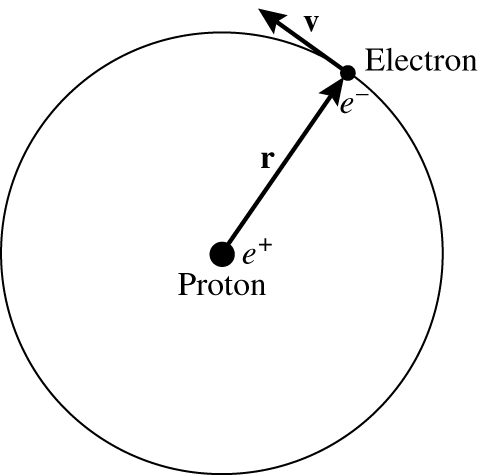
_images/Figure_5pt5.jpg — Fig. 37 The Bohr model of the hydrogen atom.#

Bohr model for hydrogen atom

In a hydrogen atom we have an electron of mass \(m\) and charge \(e^-\) in orbit around a proton of charge \(e^+\). The electron is in an allowed orbit, a distance \(r\) from the proton, and orbits with a speed \(v\) (see figure 37). We need to work out the energy of the orbit. We start by noting that the centripital force must balance against the electrostatic attraction between the electron and proton, which gives

(23)#\[\frac{Ze^2}{4\pi\epsilon_0 r^2} = \frac{mv^2}{r},\]

where \(Z\) is the atomic number (the number of protons in the nucleus, \(Z=1\) for hydrogen). Re-arranging equation (23) gives

\[\frac{1}{2}mv^2 = \frac{Ze^2}{8\pi\epsilon_0 r},\]

but \(1/2 mv^2\) is the kinetic energy of the electron, so

(24)#\[K.E = \frac{Ze^2}{8\pi\epsilon_0 r}.\]

We’re trying to work out the total energy of the orbit, so we also need to know the potential energy due to the electrostatic attraction. We can calculate the potential energy by looking at the work done assembling the atom. Start with the electron at an infinite distance from the proton, and move it a small distance \(dr\) towards the proton. The work done in moving that small distance \(dr\) is \(Fdr\), where \(F\) is the electric force on the electron. To find the potential energy of the atom, we have to add up all the work done in moving the electron from infinity to \(r\). The potential energy is then given by

\[\begin{split}\begin{align} P.E &= \int_{\infty}^r Fdr = -\int_r^{\infty} F.dr \\ &= -\int_r^{\infty} \frac{Ze^2}{4\pi\epsilon_0 r^2} dr \\ &= -\frac{Ze^2}{4\pi\epsilon_0 r}. \end{align}\end{split}\]

The total energy is the sum of the potential and kinetic energy:

(25)#\[\begin{split}\begin{align} E &= P.E + K.E \notag \\ &= \frac{Ze^2}{8\pi\epsilon_0 r} - \frac{Ze^2}{4\pi\epsilon_0 r} \notag\\ &= -\frac{Ze^2}{8\pi\epsilon_0 r}. \end{align}\end{split}\]

The total energy is negative because the electron is bound to proton; if we wish to free the electron from the proton, we must add energy. So far, our derivation has been entirely classical. We make a semi-classical model by adding Bohr’s hypothesis that the angular momentum is quantised, so

(26)#\[L = mvr = nh/2\pi,\]

where \(n=1,2,3 \ldots \infty\). We can use this to solve the radius of the electron’s orbit, \(r\). We take equation (23), which we obtained from balancing the coulomb force and centripetal acceleration, and we re-write it like so

(27)#\[\frac{4\pi\epsilon_0}{mr} (mvr)^2 = Ze^2.\]

We then substitute equation (26) for \(mvr\) in equation (27) to find

\[\frac{4\pi\epsilon_0}{mr} \left( \frac{nh}{2\pi} \right)^2 = Ze^2,\]

which can be re-arranged to give the radius of the \(n^{th}\) orbit, \(r_n\), as

(28)#\[r_n = \frac{4\pi\epsilon_0}{mZe^2} \left( \frac{nh}{2\pi} \right)^2.\]

Now we know the radius of the orbit, we can substitute this back into the equation for the total energy of the \(n^{th}\) orbit, equation (25), to find

(32)#\[E_n = -\frac{Z e^2}{8 \pi \epsilon_0 r_n} = -\frac{R^{\prime}}{n^2},\]

where \(R^{\prime}\) is given by

(30)#\[R^{\prime} = \left(\frac{\mu}{m_{e}} Z^2 \right) R_{\infty} hc.\]

Here \(R_{\infty} hc\) is the Rydberg energy (13.606 eV = \(2.18 \times 10^{-18}\) J) and μ is the reduced mass, which is

\[\mu = m_e \left( \frac{m_p}{m_e + m_p}\right) = 0.99946 m_{e}\]

for hydrogen (one electron orbiting a proton) so the effective Rydberg energy for hydrogen is

\[R_{\rm H} = \left( \frac{\mu}{m_{e}} 1^{2} \right) R_{\infty} hc = 0.99946 R_{\infty} hc.\]

Therefore, the integer \(n\), known as the principal quantum number completely determines the radius and energy of each orbit of the Bohr atom. When the electron is in the lowest energy level (\(n=1\), the ground state), its energy is simply \(E_{1}=-R_{H}\). It would take an amount of energy equal to \(R_{H}\) to remove the electron from the atom, so \(R_{H}\) is the ionisation energy of the atom. In general \(R^{\prime}\) scales with the square of the atomic number \(Z\).

Atomic lines of hydrogen#

We are now in a position to understand the lines emitted in the spectrum of hydrogen. When an electron moves between one orbit and another, it emits or absorbs a photon. The energy of the photon is given by the difference in energy between the two orbits, \(\Delta E = E_{n_1}-E_{n_2}\). Equation (32) leads to an equation for the energy of the emitted or absorbed photon

\[E_{photon} = E_{n_1} - E_{n_2} = R_{H} \left( \frac{1}{n_{1}^2} - \frac{1}{n_{2}^2} \right).\]

Since, for a photon \(E=h\nu\), the corresponding frequency of the photon is

\[\nu_{1,2} = \frac{R_{H}}{h} \left( \frac{1}{n_{1}^2} - \frac{1}{n_{2}^2} \right).\]

And, finally, we can use the wave equation \(\nu \lambda = c\) to obtain the wavelength of the photon as

(31)#\[\begin{split}\lambda_{1,2} = \frac{hc}{R_{H}} \left(\frac{1}{n_{1}^2} - \frac{1}{n_{2}^2} \right)^{-1} \\\end{split}\]

where \(R_{H}/hc= 1.09677\times10^{7}\) m^-1. These equations give the wavelengths/frequencies of the radiation that would be emitted/absorbed when electron jumps from one level to another.

When an electron jumps from the \(n=3\) orbit to \(n=2\) level, a photon of wavelength \(\lambda = \frac{hc}{R_{H}} \left( \frac{1}{4} - \frac{1}{9} \right)^{-1} = 656\) nm is emitted. The reverse process can also occur; an electron in the \(n=2\) orbit can absorb a photon of wavelength 656 nm and jump to the \(n=3\) orbit.

Hydrogen line series#

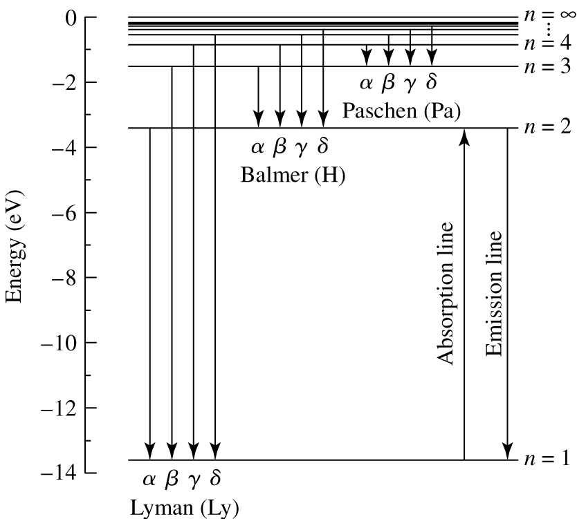
_images/Figure_5pt7.jpg — Fig. 38 Energy level diagram for a hydrogen atom showing the Lyman, Balmer and Paschen lines (downward arrows indicate emission lines; upward arrows indicate absorption lines).#

Hydrogen energy level diagram

Considering the energy levels in more detail, it is clear that the line spectrum of hydrogen will exhibit a number of “series”, associated with transitions to and from a given orbit. For example, transitions from the \(n=3,4,\ldots,\infty\) energy level to the \(n=2\) level cause a series of emission lines known as the Balmer series, often denoted with the letter H (see figure 38). The line we considered above, when the electron jumps from \(n=3\) to \(n=2\) is part of the Balmer series. In fact, it is the first line of the Balmer series, Hα. It’s wavelength of 656 nm is in the middle of the optical part of the spectrum. The Balmer series is exactly the same series of lines observed by Kirchhoff and Bunsen. There are also series of lines in the ultraviolet, corresponding to transitions to and from the \(n=1\) ground state (the Lyman series) and an infrared series of lines, corresponding to transitions to and from the \(n=3\) orbit (the Paschen series).

Look at the spacing of the energy levels in figure 38, and compare it to equation (32). As \(n\) increases, the energies of the orbits become more closely spaced. Therefore the difference in energy, or frequency, or wavelength between successive lines in a series gets smaller as \(n\) increases. Eventually, the spacing of the energy levels approaches zero, and the emission or absorption lines get very closely spaced indeed. We say the series has reached its limit.

Hydrogen-like atoms#

When we derived the energy levels for hydrogen, we set the atomic number, \(Z=1\). However, you would get a similar series of energy levels for any atom consisting of a single electron orbiting a nucleus containing \(Z>1\) protons. For example, singly ionised helium, is such an atom, with \(Z=2\). Although the energy level diagram for any hydrogen-like atom has the same form as for hydrogen, the exact spacing of the levels depends upon the atomic number, \(Z\) i.e.

(32)#\[E_n = -\frac{Z^2 R_{\rm Z}hc}{n^2},\]

where \(R_{\rm Z} h c\) = 13.6 eV. In the case of singly ionised helium, the spacing between the energy levels is four times that between the energy levels in a hydrogen atom so its ionization energy is 54.4 eV. The equivalent of Eqn. (31) for ionized helium is

\[\begin{align} \lambda_{1,2} &= \frac{1}{4} \frac{hc}{R_{He}} \left(\frac{1}{n_{1}^2} - \frac{1}{n_{2}^2} \right)^{-1}. \end{align}\]

where \(R_{He}/hc = 1.09722\times10^{7}\) m^-1 is the Rydberg constant for helium.

More complex atoms#

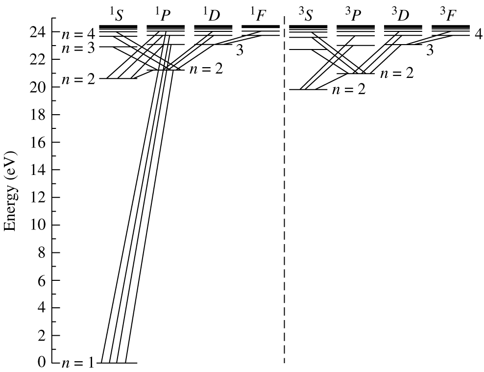
_images/Figure_5pt14.jpg — Fig. 39 Some of the energy levels of a neutral helium atom (2 protons, 2 electrons). A small number of possible transitions is also indicated.#

Energy levels of neutral helium

Bohr’s model is very successful in describing the line spectrum of hydrogen-like atoms. However, it is important to note that Bohr’s model atom is not correct. Although the angular momentum is quantised, it is not quantised in the way suggested by Neils Bohr. To some extent, it is a matter of good luck that we obtained the correct energy level diagram for hydrogen! To calculate the energy level of more complex atoms, it is necessary to use the complete quantum theory, and to account for the interactions between electrons, as well as between the electron and the nucleus. This calculation rapidly becomes extremely complex, and the number of possible energy levels grows rapidly as the number of electrons in the atom rises. Figure 39 shows a simplified energy level diagram for atomic helium. Even with a single extra electron, the energy level diagram is already much more complex, and there are many more possible transitions with corresponding emission and absorption lines.

The Kirchhoff-Bunsen laws#

We are now in a position to understand the Kirchhoff-Bunsen laws, which describe what kind of spectrum will be seen from a given source.

A hot dense gas or hot solid produces a continuum spectrum with no spectral lines – Since a solid is made of atoms, why don’t solids also emit a line spectrum? The answer is that interactions between the closely spaced atoms change the energy levels available to the electrons, so that electrons can have a large range of energies. As a result, the object can emit or absorb light across a large range of wavelengths – If the body is in thermal equilibrium, this spectrum is described by the Planck curve.
A hot, diffuse gas produces emission lines. Because the gas is hot, electrons exist in excited states. When the electrons decay to lower energy orbits the energy lost is carried away by a single photon. This photon can only have certain, discrete energies, corresponding to the differences in energy between allowed orbits.
A cool, diffuse gas in front of a continuous spectrum source (a hot solid or dense gas) produces absorption lines in the continuous spectrum. Absorption lines are produced when an electron makes a transition from a lower energy orbit to a higher energy orbit. If a photon in the continuous spectrum has exactly the right amount of energy, equal to the energy difference between two orbits, that photon can be absorbed and the electron makes the transition to a higher orbit. The cool diffuse gas thus absorbs light from the continuous spectrum, but only at discrete wavelengths. This produces an absorption line spectrum.

The use of spectral lines#

It turns out that the presence of absorption and emission lines in the spectra of astrophysical objects is one of the most powerful tools available to astronomers. We can use the lines to measure velocities, using the Doppler effect. The wavelengths of lines act as fingerprints for the material in an object. What we will look at in the next section is that the relative strengths of these absorption lines depends upon the physical properties of the emitting gas. These properties (temperature, density and pressure) can be determined by a careful examination of spectral lines. We will see that the strengths of the spectral lines (and thus the explanation for the Harvard spectral sequence) is strongly dependent on the temperature; giving us yet more ways of measuring the temperature of astrophysical objects!