
Chapter 11: Measuring mass#
Having dealt with the theory of gravity, let’s start to use it to measure mass. The mass of an object is probably the most fundamental and important measurement we can make for an object (for example, a star’s brightness, lifetime and evolution are mainly determined by its mass). In almost all cases, measuring the mass of an object involves measuring the effect of its gravity on nearby objects. We will start with a example which is close to home; the masses of planets in our solar system.
Planets in the solar system#
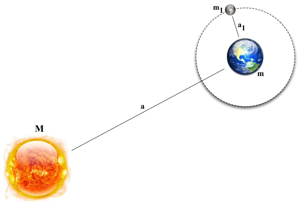
Fig. 54 Geometry of a planet with a moon, orbiting the Sun (not to scale!)#
Schematic of planet with a moon - not to scale!
If a planet has a moon orbiting it, we can use Kepler’s 3rd law to calculate the mass of the planet, relative to the mass of the Sun. Figure 54 shows the geometry. A planet of mass \(m\), orbits the Sun (mass \(M\)) with a semi-major axis of \(a\). The planet also has a moon, with a mass \(m_1\), which orbits the planet with a semi-major axis \(a_1\). Using Kepler’s 3rd law as written in equation (40), we find the following equation for the period of the planet’s orbit around the Sun
and a corresponding equation for the period of the moon’s orbit around the planet
We divide the two equations to get
But here we can use a (very good) approximation. Since the mass of the moon is much less than the mass of the planet (the Moon is around 1% the mass of the Earth), we have \(1+m_1/m \approx 1\), and using the same argument for the planet and Sun, \(1+m/M \approx 1\). Re-arranging, we find
Thus the relative mass of any planet with a moon can be found once the periods and semi-major axes of the moon and planet are known. The periods are easy to measure by tracking the motion of planets in the night sky, and the same data can yield distances using the parallax method.
Absolute planetary masses#
The equation above yields the masses of the planets in the Solar system, relative to the mass of the Sun, \(M\). If we could measure the absolute mass of a single planet, we can find the mass of the Sun from \(M = m_p / \frac{m_p}{M}\). In a rare case of astronomy progressing by experiment, the mass of the Earth was measured in a beautiful experiment by Henry Cavendish in 1798 (more than 100 years after the Principia was published).

Fig. 55 A sketch of Cavendish’s experiment to measure the mass of the Earth#
Sketch of Cavendish’s experiment
Cavendish’s experiment is shown (in sketch form) in figure 55. He attached a bar holding small masses to a torsion wire and placed two much larger masses close by. The large masses were equidistant from the smaller, test masses - a distance \(r\). By considering the forces on the small masses due to the large masses, and the Earth, Cavendish could calculate the mass of the Earth.
The force on the test masses due to the large masses is
and the force on the test masses due to the Earth is
Dividing equation (44) by equation (43) gives
or
All of the quantities on the right hand side of equation (45) can be measured. \(F_p\) is measured from the twist of the torsion wire. \(F_E = ma\) can be measured by measuring the gravitational acceleration of the test particles when dropped – The distance \(s\) travelled in a time \(t\), under constant acceleration \(a\) is \(s=at^2/2\) – The radius of the Earth is easily measured using geometrical techniques.
In this way, Cavendish determined the mass of the Earth, and hence the absolute mass of all planets. Cavendish’s equipment was remarkably sensitive. The force involved in twisting the torsion balance was very small, roughly equivalent to the weight of a large grain of sand. To prevent air currents and temperature changes from interfering with the measurements, Cavendish placed the entire apparatus in a wooden box about 0.6 m thick, 3 m tall, and 3 m wide, all in a closed shed on his estate. Through two holes in the walls of the shed, Cavendish used telescopes to observe the movement of the torsion balance’s horizontal rod. The motion of the rod was only about 4mm, and Cavendish had to account for the constant swaying of the rod, which was never still. Cavendish’s experiment was repeated many times, but his accuracy wasn’t bettered for nearly 100 years.
Stellar masses#
It is phenomenal to consider that we can measure the mass of stars so impossibly distant that the light we see from them is hundreds of years old. All of the direct measurements of stellar masses we have come from stars in multiple systems; a collection of stars bound together by their own gravity. The most important of these are the binary stars - two stars which orbit each other around a common centre of mass. Binary stars are surprisingly common: over half of the stars visible to the naked eye are actually in binary systems. Binary systems are classified according to their observational characteristics. Different types of binary systems provide different ways of measuring mass, and some types of binary system allow a rich set of data to be collected. In the sections that follow, we will consider some types of binary star in turn.
Visual Binaries#
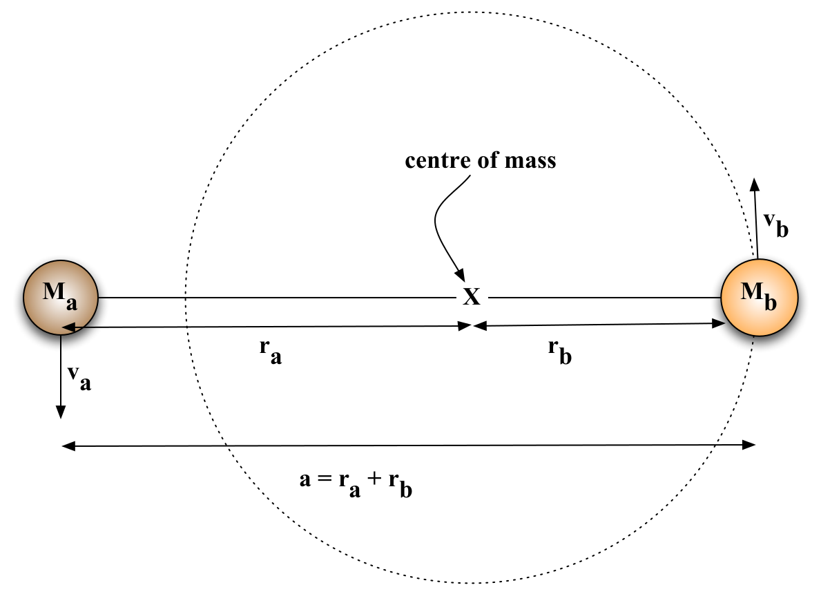
Fig. 56 Circular orbits around the centre of mass (COM). The centre of mass is marked with a cross, whilst the circular orbit of star b around the COM is shown as a dotted line.#
Circular orbits of two stars
Remember that the resolving power of a telescope is not infinite; in practise an image taken from a ground based telescope has an image quality dictated by the atmosphere. This is called seeing, and means that the typical size of a stellar disc in a ground-based image is around one arcsecond – Space-based telescopes can do rather better, being above the atmosphere and hence limited by their optics – Therefore, if the two stars in a binary are very close together, so that their separation on the sky is less than an arcsecond, the light from the stars will be blurred together. We will not see the stars as a binary system at all; such a binary system is unresolved.
Binaries in which we can clearly see both components are called visual binaries. For a star to be a visual binary the components must be widely separated, and both components must be bright enough to detect. Visual binaries are very useful for measuring masses simply, with a minimum of observations.
In some visual binaries, we are fortunate that the orbital period is short enough that we can actually watch the stars move around their orbits. By patiently watching visual binaries, we can measure the size of the orbits. Figure 56 shows the geometry of a binary star system with circular orbits. From the definition of the centre of mass, we know that the sizes of the star’s orbits \(r_a\) and \(r_b\), are related through
Therefore the mass ratio (\(m_a/m_b\)) is given by
From our images, we can measure the angular sizes of the orbits \(\alpha_a\), \(\alpha_b\). Since these angles are small, they are related to the sizes of the orbits by \(r_a = d\alpha_a\) and \(r_b = d\alpha_b\), where \(d\) is the distance to the binary. As a result, the mass ratio is given by
and can be found by a simple measurement of the angular sizes of the orbits, without knowing the distance to the stars.
If the distance is known (e.g. from a measured parallax), we can calculate the physical sizes of the orbits, \(r_a\) and \(r_b\). It follows that we can also measure the binary separation, \(a=r_a+r_b\) and use this in Kepler’s third law to find the total mass of the binary, since
and \(P\) is also directly measured from the star’s orbit. Once we know the mass ratio, and the total mass, we can find the individual masses through some simple algebra. You should be able to convince yourselves that
Since all the terms on the right hand side of this equation can be measured, it follows we can measure individual masses of stars within a visual binary system, armed with nothing more than images of the stars as they orbit the centre of mass, and a distance to the binary!
Orbital Inclination#
Our discussion of using visual binaries to measure mass above presents quite a simplified picture. In reality, the analysis of the data is more complex because we do not know the inclination of the binary orbit to our line of site. The true situation is shown in figure 57.
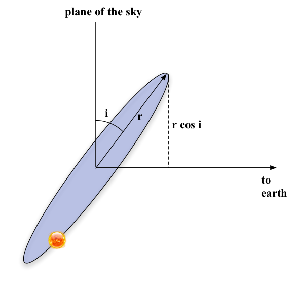
Fig. 57 An orbit inclined with respect to our line of sight. The angle \(i\) between the orbit and the plane of the sky is called the orbital inclination. We do not see the true orbit, instead we see the orbit projected on the plane of the sky.#
Orbit inclined to our line of sight
When we track the motion of stars in a visual binary, we do not see the true orbit, but the projection of the orbit onto the plane of the sky. Instead of measuring the true sizes of the orbits \(r_a\) and \(r_b\) we instead measure the projected sizes, for example \(r_a^{\prime} = r_a\cos i\). We can still measure the mass ratio without knowing the inclination because
We do, however, need to know the orbital inclination to measure the total mass, as
where \(\alpha^{\prime} = \alpha_a^{\prime} + \alpha_b^{\prime}\) is the projected angular separation of the binary.
Therefore, whilst a visual binary can yield the mass ratio without knowing the orbital inclination or distance, a full solution for the individual masses needs knowledge of both the orbital inclination and distance to the binary. We might measure the distance using a parallax measurement, but how to measure the orbital inclination? It turns out that very detailed observations of the binary star orbits can tell us the orbital inclination as well.
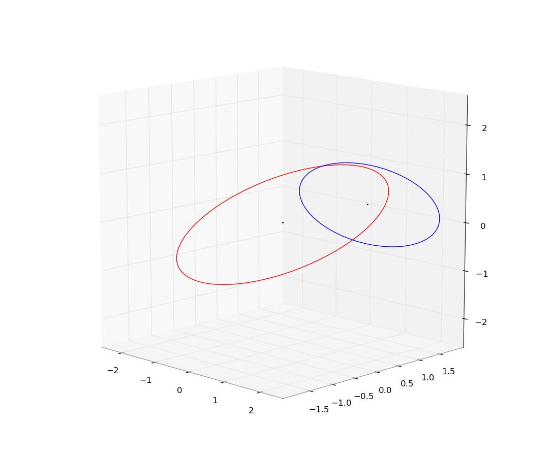
Fig. 58 The projection of an inclined, circular orbit onto the plane of the sky. A circular orbit (red) is inclined to our line of sight by 60 degrees. It’s projection on the sky (blue) is an ellipse. The centre of the circular orbit projects to the centre of the ellipse (both marked by dots).#
Projection of an inclined circular orbit onto plane of sky
Figure 58 shows the basic idea. A circular orbit (shown in red) is inclined to our line of sight at 60 degrees. It’s projection onto the plane of the sky is an ellipse. Therefore, a star on this orbit appears to follow an elliptical orbit. However, if the orbit is measured accurately, it is clear that something is not right. The star orbits on an elliptical orbit, but the centre of the orbit is not at one of the focii of the ellipse. Instead, the centre of the orbit is in the centre of the ellipse. Thus, the star appears to violate Kepler’s first law! Therefore the inclination of the true orbit can be determined by comparing the observed stellar positions with mathematical projections of various orbits onto the plane of the sky.
Therefore, detailed measurements of the orbits of visual binaries can be used to measure the mass ratio, and the inclination of the binary orbit. Combined with a distance measurement, the total mass of the binary (and hence the individual stellar masses) can also be determined.
A visual binary case study: Sirius#
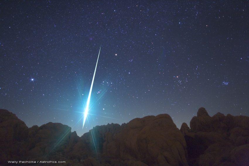
Fig. 59 A bright Geminid meteor, and Sirius (the bright star in the bottom left).#
Bright Geminid meteor and Sirius in the bottom left
We need not look far for an example of a visual binary. Sirius is the brightest star in the night sky (figure 59); and in many ways is the archetypical visual binary. Sirius consists of two stars, separated by around 7.5 arcseconds. The brightest star, Sirius A has a luminosity of 25.4 \(L_{\odot}\) and an effective temperature of 9,940 K. In many ways it is a typical star of spectral type A2. Sirius B is much hotter, at 25,200 K but much fainter, with a luminosity of 0.026 \(L_{\odot}\). Since, for a black body, \(L=4\pi R^2 \sigma T_{eff}^4\), we can immediately tell that Sirius B is much smaller than Sirius A; in fact it is over 200 times smaller.
Sirius is extremely bright because in part because it is close to us. It’s therefore not suprising that it shows a large proper motion. The motion of Sirius A and B in the sky is shown in figure 60. As well as a large proper motion relative to the background stars, the paths of the stars also reveal the motions of the two stars around the centre of gravity.
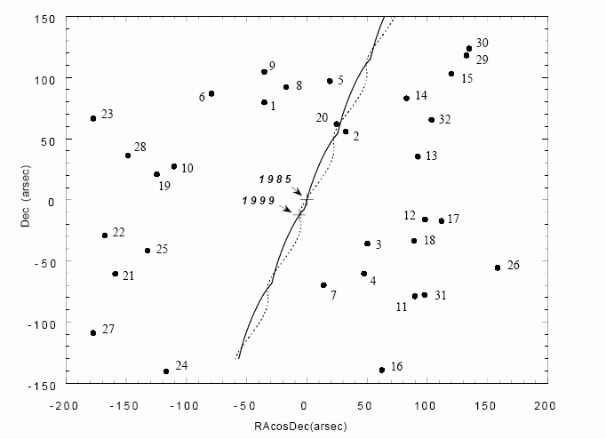
Fig. 60 The paths of Sirius A (solid line) and Sirius B (dashed line) in the sky. Background stars are marked with dots and numbers. On top of the binary motion, there is a very large proper motion.#
Paths of Sirius A and B in the sky
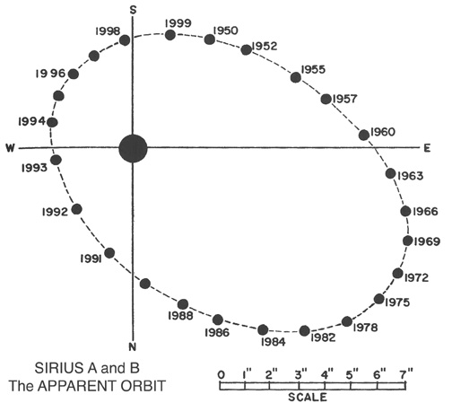
Fig. 61 The ’apparent’ orbit of Sirius B. This is the orbital motion of Sirius B after subtracting the proper motion of the binary, and the motion of Sirius A.#
Apparent orbit of Sirius B
Figure 61 shows the motions of Sirius A and Sirius B again, but this time the proper motion, and the motion of Sirius A have been subtracted, so Sirius A appears stationary. This makes the orbit of Sirius B more obvious. The orbit is elliptical, but is not centred on one of the focii of the ellipse. This tells us the orbit is inclined at an angle to our line of sight. Detailed analysis of the orbital shape reveals that the orbital inclination of Sirius AB is roughly 44 degrees. The size of the orbit is \(\alpha = 7.56\) arcseconds. Parallax measurements reveal the distance to the binary is \(d=2.6\) parsecs. The size of the orbit is thus given by \(a=\alpha d = 19.7\) AU. We can apply Kepler’s third law to find the total mass of the binary - about 3 Solar masses.
Look again at the orbits of Sirius A and B in figure 60. It is clear that the orbit of Sirius A is about half the size of Sirius B’s orbit. Since
we can immediately see that Sirius A is roughly twice as massive as Sirius B. Since the total mass of Sirius AB is 3 Solar masses it follows that Sirius A is roughly 2 Solar masses and Sirius B is roughly the same mass as the Sun.
Whilst Sirius A is essentially a normal star of spectral type A2, with a typical mass and luminosity, Sirius B is very odd indeed. It has roughly the same mass as the Sun, is nearly four times hotter than the Sun and yet its radius is 200 times smaller than a typical A2 star. That means the radius of Sirius B is much around the same as that of the Earth! Sirius B is one of the earliest known White Dwarfs, extremely dense stars which are the ultimate fate of stars like our Sun. They are formed from the hot dense core of the star as it reaches the end of its life.
The extremely high density of white dwarfs can only be supported against gravitational collapse due to electron degeneracy pressure; a curious quirk of quantum mechanics. The Heisenberg uncertainty principle states that you cannot simultaneously define the position and momentum of an electron to arbitrary precision. If the position is known more accurately, the momentum becomes more uncertain, and vice versa. In a white dwarf, the electrons are confined within a very small radius. Their positions are thus well known, so their momenta must be very uncertain! This means that some electrons will have high momenta, and be moving at high speeds. Just like a gas in a box, high electron speeds cause a pressure, which supports the white dwarf against gravity.