Chapter 9: Line strength

Chapter 9: Line strength#

In the last section we dealt with two of the puzzles arising from early astronomical spectroscopy. Now, we turn to the last puzzle - the Harvard spectral classification sequence.

The Harvard sequence in more detail#

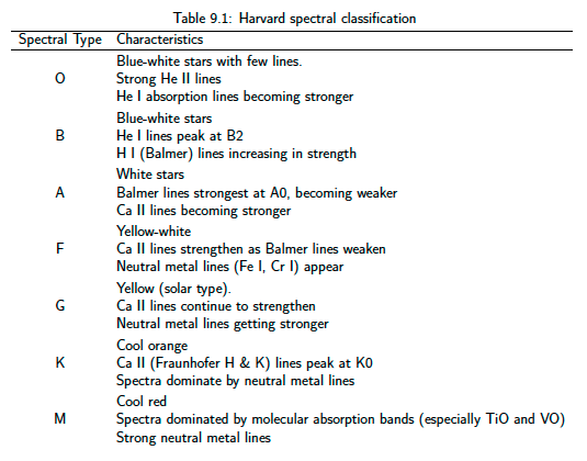
_images/Table9-Harvard.png — Fig. 40 Harvard spectral classification#

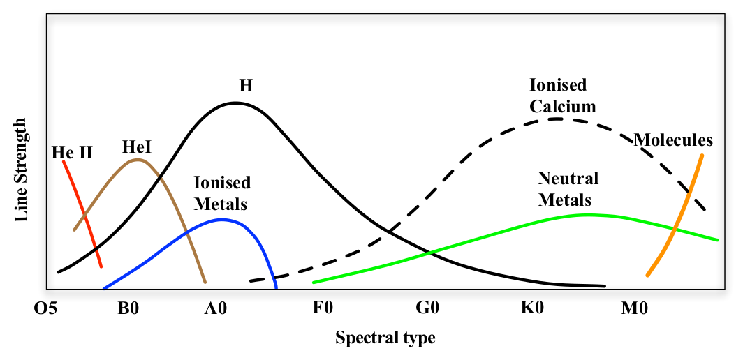
_images/harvard_sequence2.png — Fig. 41 A crude sketch of the variation of line strength along the Harvard spectral classification sequence, at the level you are expected to remember it for this course.#

Coarse sketch of variation in line strength across Harvard spectral sequence

The Harvard sequence classifies stars according to the strength of their absorption lines. There are various ways of presenting this information. In figure 40 a.k.a. Table 9.1 I present a summary of the trends in text form – Note that in the table the term metal is used to denote any element heavier than helium. This is a standard convention in astronomy. It arises because hydrogen and helium are by far the most abundant elements in the Universe – Figure 41 shows the important trends in line strength in a graphical sketch.

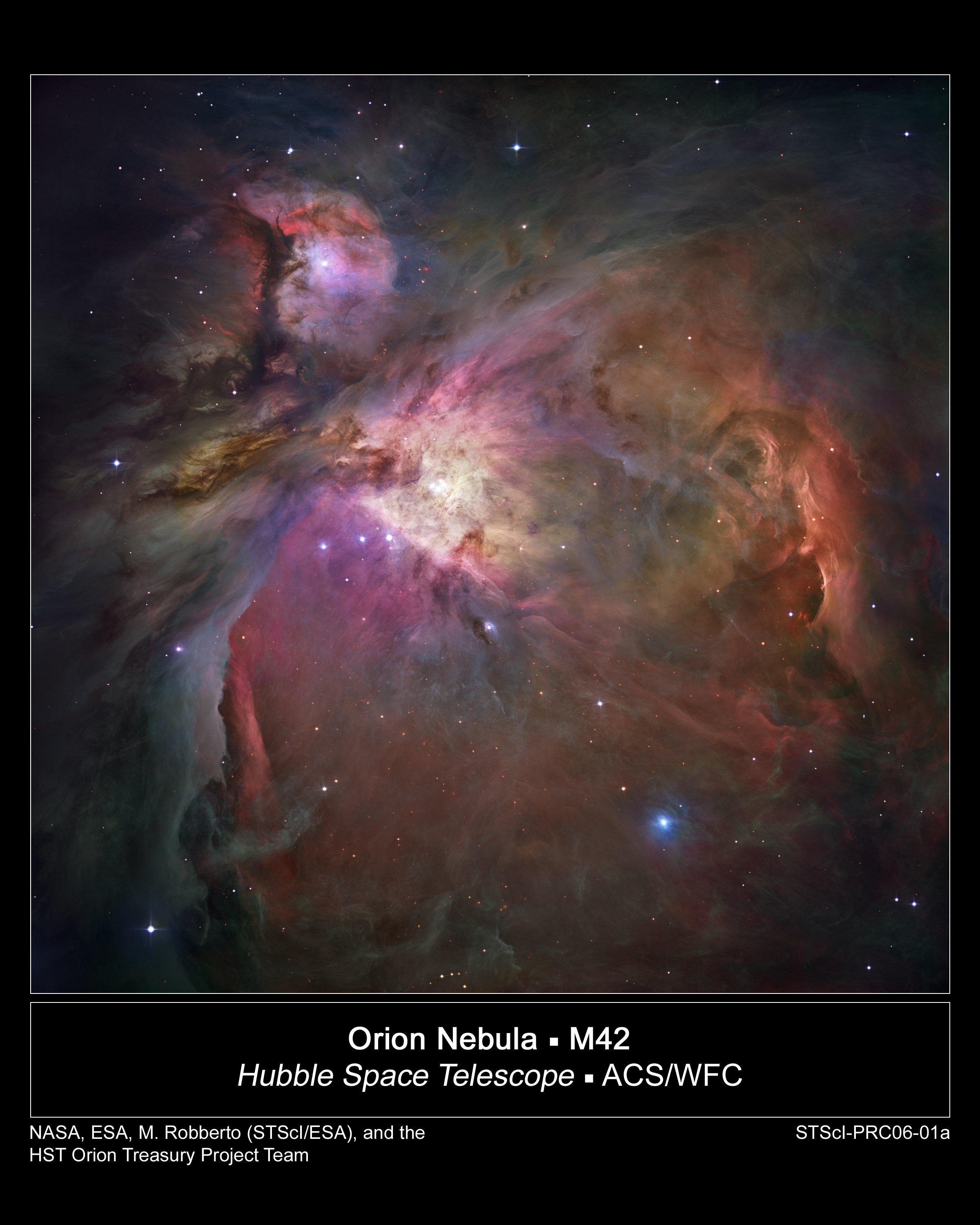
_images/orion_nebula.jpg — Fig. 42 The Orion Nebula, as seen from the Hubble Space Telescope. More than three thousand stars appear in this image, with spectral types ranging from mid-O to early-M. This is despite all these stars being formed from the same cloud of gas and dust.#

Orion Nebula

What is the physical basis for the Harvard sequence? Since it is based on absorption line strengths, we must try and understand what controls the absorption line strength in stars. Why does one star have strong hydrogen lines, and another have weak hydrogen lines? Our first guess might be that it is related to the abundance of hydrogen in the star’s photosphere. Some easy observations show that this is not the case; figure 42 shows the Orion nebula. Located halfway down Orion’s sword, this cloud of dust and gas is a stellar nursery. The stars we see here are only a million years old. Crucially, they have all formed from the same cloud of gas, and so we expect them to have the same composition. Nevertheless, the familiar Harvard sequence can still be seen in the young stars of Orion. So the abundance of elements in stars is not the primary cause of their line strength variations.

Line strengths#

To see what factors control line strengths consider the first line of the Balmer series, Hα. An Hα absorption line is caused by an electron absorbing a photon and moving from the \(n=2\) energy level to the \(n=3\) level. Of course, for this to occur means that some electrons had to be in the \(n=2\) energy level in the first place. Since an excited electron will tend to decay into the ground state (\(n=1\)), how do the electrons get into the \(n=2\) level in the first place?

Electrons can be excited into higher energy levels by two mechanisms. As we have seen, they can absorb photons of the correct energy. This process is particularly important in stellar atmospheres. Collisions between atoms can also excite electrons by passing energy from one atom to another. Both of these processes depend upon the temperature; the higher the temperature, the higher the mean energy of atoms and photons, and more photons or atoms are capable of exciting electrons. Therefore, we might expect the number of electrons in the \(n=2\) energy level of hydrogen to increase with increasing temperature.

The Boltzmann equation#

To understand this process in a quantative way, we need to return to statistical physics, which we discussed earlier. Remember that, in thermal equlibrium, the probability of a particle having energy E was given by

\[P(E) \propto e^{-E/kT}.\]

If we are comparing two energy levels (labelled 1 and 2), then the ratio of the probability \(P_2\) that an electron is in level 2 to the probability \(P_1\) that an electron is in level 1 is given by

\[\frac{P_2}{P_1} = \frac{e^{-E_2/kT}}{e^{-E_1/kT}} = e^{-(E_2-E_1)/kT}.\]

Suppose \(E_2\) is greater than \(E_1\). Therefore, as the temperature tends towards zero, the quantity \(-(E_2-E_1)/kT\) tends towards \(-\infty\), and \(P_2/P_1\) tends towards zero. In this case, all the electrons would be in level 1. However, as the temperature increases, the proportion of electrons in energy level 2also increases.

In many atoms, there may exist many quantum states available to an electron which have the same energy. These quantum states are said to be degenerate. We define \(g_n\) to be the number of states with energy \(E_n\). Then, the ratio of the probability that an electron will be found in any of the \(g_2\) states with energy \(E_2\), to the probability that it will be found in any of the \(g_1\) states with energy \(E_1\) is given by

\[\frac{P(E_2)}{P(E_1)} = e^{-(E_2-E_1)/kT}.\]

Since astronomical objects contain very large numbers of atoms, the number of atoms \(N_2\) with energy \(E_2\) is indistinguishable from the probability that an atom has energy \(E_2\). Thus, the ratio of the numbers of atoms in one energy level to another is given by the Boltzmann equation

(33)#\[\frac{N(E_2)}{N(E_1)} = \frac{g_2}{g_1} e^{-(E_2-E_1)/kT}.\]

The Boltzmann equation can also be expressed in logarithmic units,

\[\log \frac{N(E_2)}{N(E_1)} = \log \frac{g_2}{g_1} -\frac{5040}{T} (E_2-E_1)\]

where \(E_2 - E_1\) is expressed in terms of electron volts (eV), since \(k = 8.62 \times 10^{-5}\) eV/K.

Let’s look at a specific example of the Boltzmann equation, and work out the relative populations of the \(n=2\) and \(n=1\) energy levels in hydrogen for the Solar photosphere. Recall from last week that the energy of a electron orbit with quantum number \(n\) was given by

\[E_n = -\frac{W}{n^2},\]

where W is the ionisation energy of the atom (13.6 eV for hydrogen). We also need to know the degeneracy of the \(n=2\) and \(n=1\) levels. For this we need the full quantum mechanical theory, but I’ll simply state there are 2 quantum states with energy \(E_1\) and 8 quantum states with energy \(E_2\). Therefore the number of electrons in state \(n=2\), divided by the number of electrons in state \(n=1\) is given by

\[\log \frac{N(E_2)}{N(E_1)} = \log \frac{8}{2} -\frac{5040}{5777} \times 13.6 \times \left( \frac{1}{1^2} - \frac{1}{2^2} \right)\]

or

\[\frac{N(E_2)}{N(E_1)} = 0.000000005\]

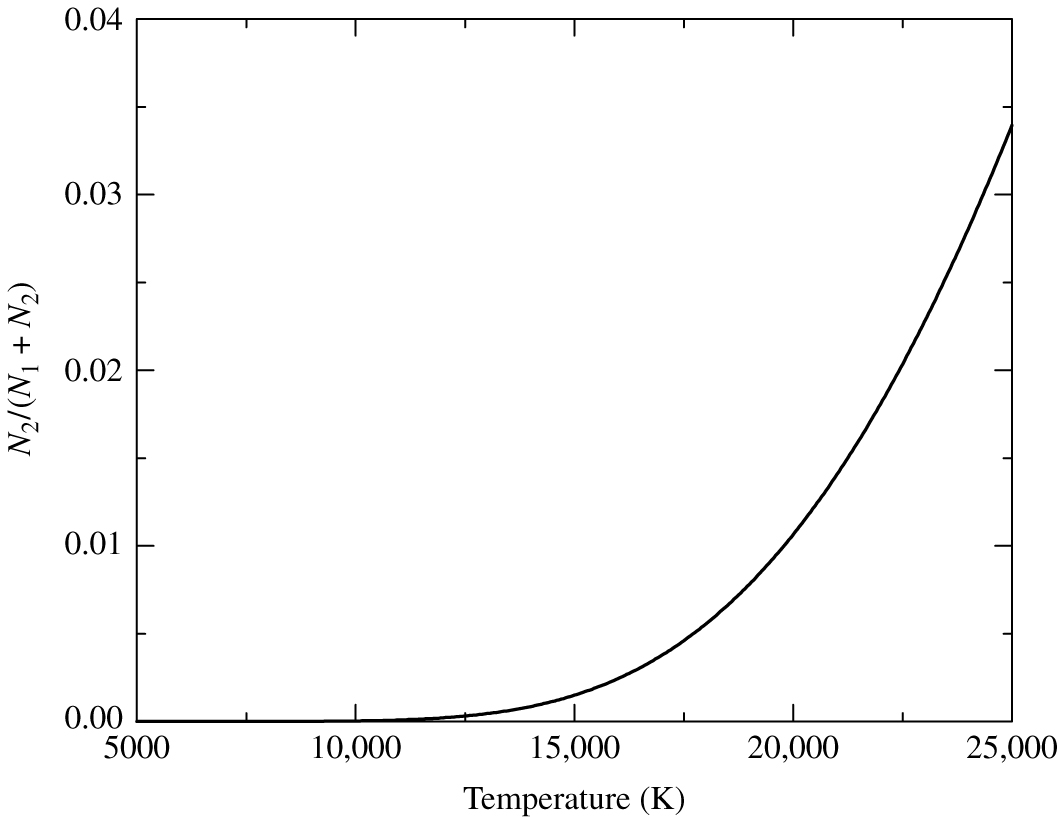
_images/Figure_8pt7.jpg — Fig. 43 The number of electrons in \(n=2\) (\(N_2\)) divided by the total number of electrons \(N_1 + N_2\) for hydrogen gas, as determined by the Boltzmann equation.#

Temperature dependence of excited electrons using Boltzmann equation

Figure 43 shows the number of electrons in energy level \(n=2\), divided by the total number of electrons, derived using the formula above. We can see that the number of electrons in \(n=2\) is a rapidly rising function of temperature.

This provides us with something of a puzzle. Recall that the Balmer lines are produced by electrons in the \(n=2\) level absorbing photons. The Balmer lines reach their peak strength at spectral types A0, corresponding to temperatures of \(\sim 9500\) K. Clearly, according to the Boltzmann equation, at temperatures higher than 9500 K an even greater number of electrons will be excited to the \(n=2\) level. If this is the case, why do the Balmer lines decrease in strength towards the hotter O and B stars?

The Saha equation#

The answer lies in the considering the number of atoms in different states of ionisation. Consider the ionisation of a species I

\[A ^I + h\nu \rightleftharpoons A^{I+1} + e^-,\]

where \(h\nu > E_I\), the ionisation energy of the species I. Clearly, as the temperature increases, the number of photons with \(h\nu > E_I\) will increase and the degree of ionisation of an element will increase correspondingly. This is why the Balmer lines decrease in strength above \(T\sim 9500\) K; it is due to the rapid ionisation of hydrogen above 1000 K. This process is illustrated in figure 44.

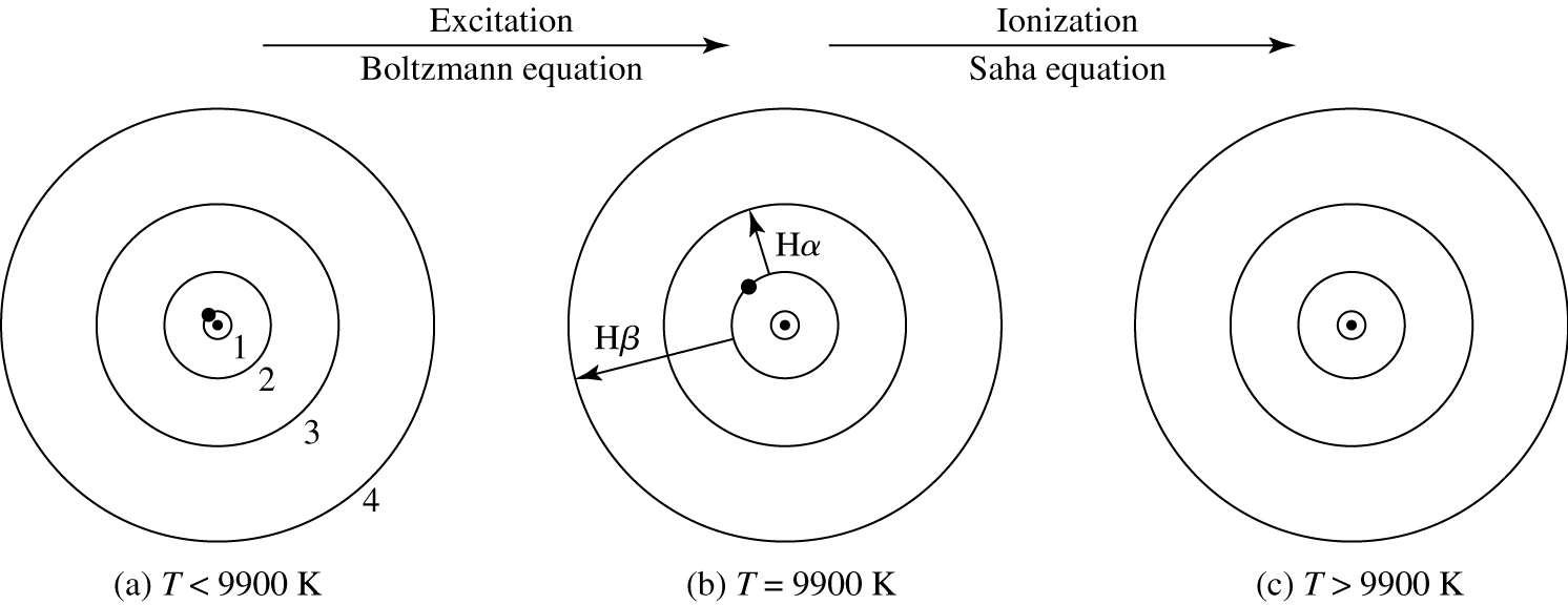
_images/Figure_8pt10.jpg — Fig. 44 The electron’s position in the hydrogen atom at different temperatures. In (a), the electron is in the ground state. Balmer absorption lines can only be produced when the electron is excited to the \(n=2\) level, as shown in (b). In (c) the atom has been ionised, and no longer produces absorption lines.#

Electrons in hydrogen at different tempertures

Just as we did for electron excitation above, we can apply statistical physics to the process of ionisation to derive the Saha equation

(34)#\[\frac{N^{I+1}}{N^I} = \frac{2}{N_e} \frac{Z^{I+1}}{Z^I} \left( \frac{2\pi m_e kT}{h^2} \right)^{3/2} e^{-E_I/kT}.\]

Since the derivation of this equation is beyond us, at least we can examine it to see if it makes intuitive sense. The Saha equation is proportional to \(e^{-E_I/kT}\); we should now expect this from our familiarity with statistical physics. The electron density \(N_e\) also enters the equation. This is not too surprising. Ionisation involves the creation of a free electron. The more free electrons that are present, the more likely an ionised atom is to capture an electron. Therefore the amount of ionisation should decrease as the electron density increases. This is what we see in the Saha equation. The term \(Z^{I}\) also appears in the Saha equation. This is a quantity known as the partition function. It represents a weighted sum of the number of ways a species can arrange its electrons with the same energy, with more energetic (and hence less likely) configurations receiving less weight. One very important point to keep in mind; all of these results in statistical physics assume thermal equilibrium. The Saha equation, like the Boltzmann equation, is only strictly valid for systems in thermal equilibrium.

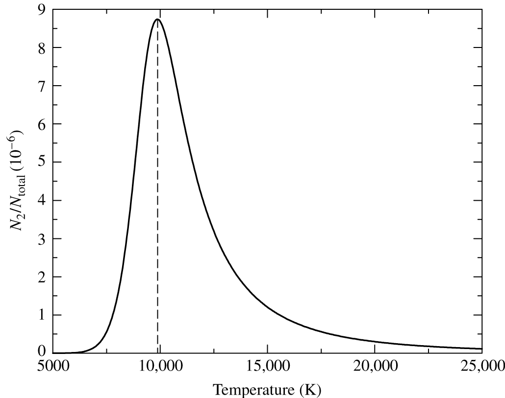
_images/Figure_8pt9.jpg — Fig. 45 The number of electrons in the \(n=2\) level of hydrogen, divided by the total number of hydrogen atoms. This calculation takes account of electron excitation (the Boltzmann equation) and ionisation (the Saha equation). The peak occurs at approximately 9900 K, in good agreement with the temperature of early-A stars, where the Balmer line strength peaks.#

Wlectrons in n=2 level of hydrogen as a fraction of the total

If we combine the Saha and Boltzmann equations, we can calculate the number of electrons in the \(n=2\) level of hydrogen as a function of temperature. The results are shown in figure 45. The number of electrons in the \(n=2\) level peaks around 9900 K. This is in reasonable agreement with the temperature of A0 stars (around 9500 K), where the Balmer line strength peaks.

A physical interpretation of the Harvard sequence#

Finally, we are in a position to understand the Harvard spectral sequence as a sequence in temperature. The line strengths of species vary along the sequence due to the interplay of electron excitation and ionisation.

Balmer lines of hydrogen - at low temperatures (spectral types K to A) the excitation effect dominates and line strength rises as the population of the \(n=2\) energy level rises. However, at high temperatures (spectral types A to O) the ionisation of hydrogen increases and the Balmer line strength drops.
Metal lines - at low temperatures (spectral types M to G), lines from neutral metals dominate, but neutral metal line strengths (e.g. Ca I, Fe I) decrease from K to G as the gas becomes ionised. From spectral types G to A the lines from singly ionised metals (e.g Mg II, Si II) become more prominent as the temperature rises and ionisation increases but eventually the gas becomes even more highly ionised and these lines also decrease in strength between spectral types A and B. Some metals (i.e Fe and Ca) have quite low ionisation energies and Ca II lines are strong between G and M-type stars.
Molecular bands - the M stars are dominated by molecular bands, especially those from titanium oxide (TiO) and vanadium oxide (VO). The generally become weaker as the temperature increases because those molecules are dissociated to form atoms of Ti, V and O. Like excitation and ionisation, dissociation can also occur due to collisions or the absorption of photons.

Stellar temperatures re-visited#

The Saha and Boltzmann equations give us two more ways of measuring the temperature of the stellar photosphere. Remember, the photospheric temperature can be derived from the peak of the continuum spectra (the Wien temperature), or from measurements of the flux at two wavelengths (the colour temperature), or from the bolometric luminosity and distance (the effective temperature).

Measurements of line strengths give us two more ways of measuring the photospheric temperature. The excitation temperature is measured from the Boltzmann equation, after using the relative line strengths to measure the population of electrons in different excited strengths. The ionisation temperature is measured from the relative populations in different ionisation stages (for example He I and He II), using the Saha equation.

Table 1 Different temperature estimates of the Sun’s photosphere#
Method	Temperature
Colour temperature	5640 K
Wien temperature	6200 K
Effective temperature	5778 K
Excitation temperature	5600 K
Ionisation temperature	6200 K

Table 1 shows the temperature of the Sun’s photosphere, measured using some of these techniques. The temperature measurements do not agree with each other, which by now should come as no surprise to you. All of these temperature estimates are only approximate, because they all assume the Sun’s photosphere is in perfect thermal equilibrium, which is not true!

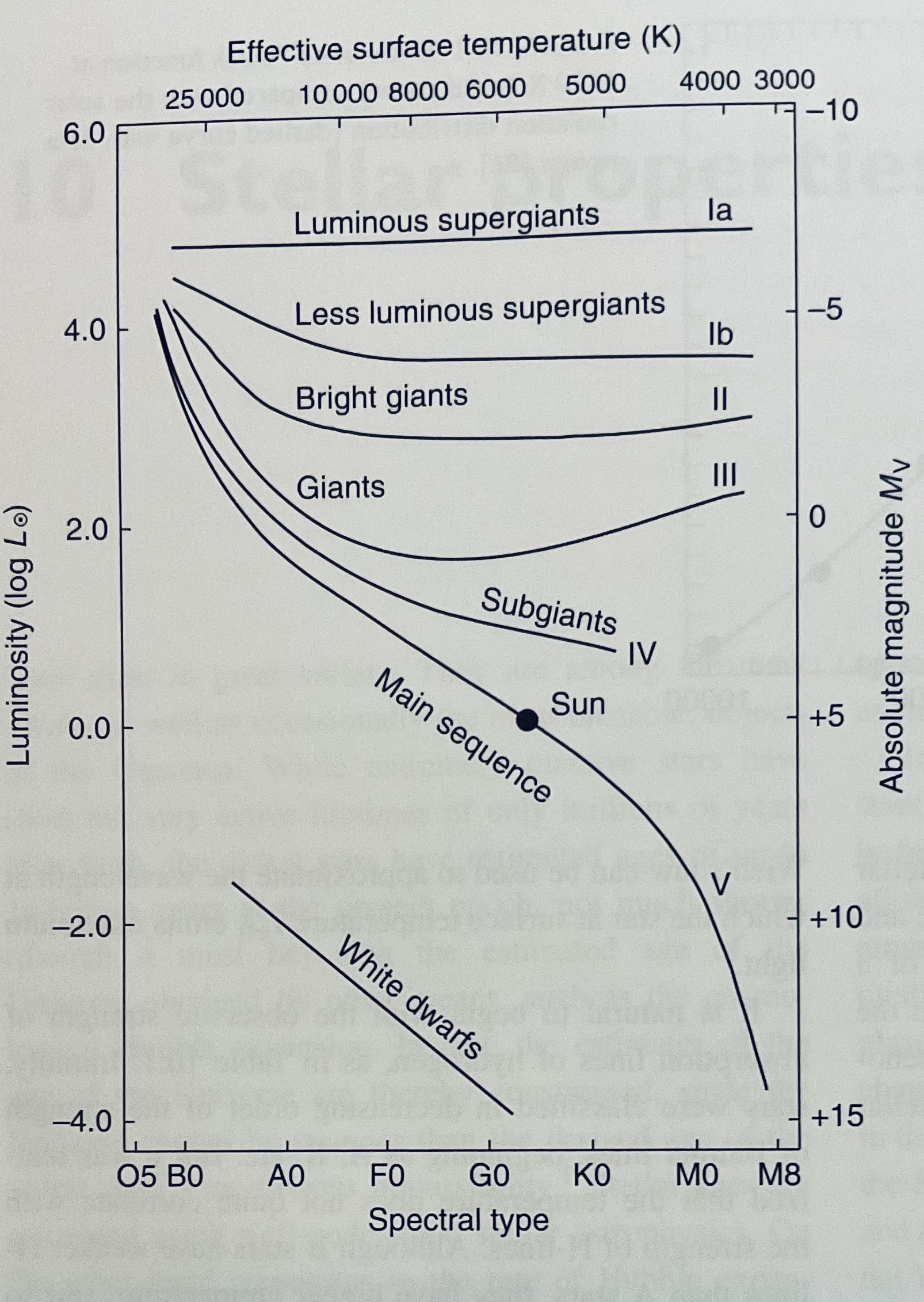
_images/PradhanHRD.jpg — Fig. 46 Hertzsprung-Russell diagram highlighting different luminosity classes, spanning supergiants (I), giants (III), dwarfs (V, main sequence) plus white dwarfs. Figure is from Pradhan & Nahar (2011, CUP).#

HR diagram

Ionization balance in stellar photospheres as described by the Saha equation (Eqn (34)) depends on electron density as well as electron temperature. Chapter 7 focused on spectral types, but classification is a two dimensional system involving spectral type (e.g. G2 for Sun) and luminosity class (V for Sun). The second criteria, introduced by Morgan, Keenan and Kellman in the 1940s, reflects spectroscopic differences in electron density (or more commonly electron pressure) between stars of the same spectral type, i.e. stars with high pressures (e.g. white dwarfs) require higher temperatures than those with low pressures (e.g. supergiants). Fig. 46 shows a Hertzsprung-Russell diagram in which main sequence stars, also known as as dwarfs have luminosity class V, giants have luminosity class III and supergiants have luminosity class I.

Abundances from line strengths#

Once the line strength variations due to temperature have been accounted for, it turns out we can see line strength variations caused by differences in the abundances of elements in the stellar photosphere. It was found that differences in the abundances of main sequence stars of the same population were very small. By the far the most abundant element is hydrogen; the abundances of elements in the Sun are shown in Table y2. Cecilia Payne (later Payne-Gaposchkin) pictured in Fig. 47 first established that stars were primarily composed of hydrogen in her PhD thesis, described by Otto Struve as “undoubtedly the most brilliant PhD thesis ever written in astronomy”.

Table 2 Solar abundances by mass#
Element	Abundance
H	73.4%
He	24.9%
C	0.29%
N	0.10%
O	0.77%
Fe	0.16%

However, there are abundance variations between stars. Stars in the haloes of galaxies (Population II stars) have lower metal abundances than stars in the disk (Population I stars). This observation allowed astronomers to realise that the Population II stars are an older generation than the Population I stars. The most metal-poor stars known have elemental abundances of heavy elements (e.g. iron) up to a million times lower than the Sun (e.g. halo star SMSS J160540.18-144323.1, according to Nordlander et al. 2019). The first or ‘primordial’ stars, composed of exclusively hydrogen and helium, are known as Population III stars, although none have yet been unambiguously discovered (JWST observations of some high redshift galaxies have hinted at the possibility of hosting Pop III stars).

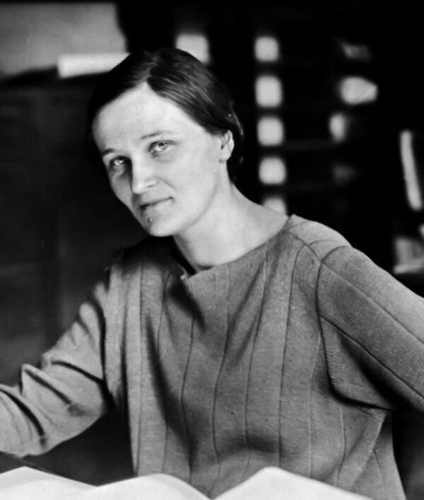
_images/payne.jpeg — Fig. 47 Cecilia Payne first established that stars were primarily composed of hydrogen in her ground-breaking PhD thesis.#

Cecilia Payne